A Crash Course on Python DataFrames

In this tutorial we’ll build on your basic Python skills and immediately start working with a new kind of object: DataFrame. We’ll meet the first Python library we’ll use throughout the course polars and walkthrough all the basics in this notebook.

Polars is very user-friendly DataFrame library for working with structured data in Python, but also R and other languages.

NoteAn alternative Python library we won’t use: pandas

As you learn more Python and grow your skills, you’ll come across or hear about Pandas probably the most popular library for working with DataFrames in Python. Many statistics courses will have you learn Pandas instead, given how long it’s been around and the wealth of materials available for learning it.

Unfortunately, Pandas is “showing its age” - it’s gone through so many changes and updates, that frankly even Eshin finds it difficult to keep up with the “right way” to do things in Pandas. Because Pandas meets so many different needs for so many different analysts (e.g. economics, finance, psych) - for the type of analyses we in Psych/Neuro/Cogsci are likely to perform on DataFrames - it gets in the way of learning and thinking.

Polars by comparison is quite a bit newer, but contains all the functionality you’ll need, while being much easier to wrap your head around. This will be a learning experience for both you and your instructors - but we strongly believe the alternatives will be unnecessarily challenging on your statistics journey.

How to use this notebook

This notebook is designed for you to work through at your own pace or use as a reference with other materials.

As you go through this notebook, you should regularly refer to the polars documentation to look things up and general help. Try experimenting by creating new code cells and playing around with the demonstrated functionality.

Remember to use help() from within this notebook to look up how functionality works.

How to import Polars

We can make polars available by using the import statement. It’s convention to import polars in the following way:

import polars as pl

Why use Polars?

So far we’ve made most use of Python lists and NumPy arrays. But in practice you’re probably working with some kind of structured data, i.e. spreadsheet-style data with columns and rows

In Polars we call this a DataFrame, a 2d table with rows and columns of different types of data (e.g. strings, numbers, etc).

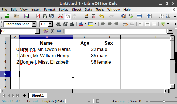
Each column of a DataFrame contains the same type of data. Let’s look at an example by loading a file with the pl.read_csv() function.

This will return a DataFrame we can check out:

df = pl.read_csv('data/example.csv')
df

shape: (3, 3)

Name	Age	Sex
str	i64	str
"Braund, Mr. Owen Harris"	22	"male"
"Allen, Mr. William Henry"	35	"male"
"Bonnell, Miss. Elizabeth"	58	"female"

Notice how Polars tells us the type of each column below it’s name.

DataFrame fundamentals

We can get basic information about a DataFrame by accessing its attributes using . syntax without () at the end:

df.shape

(3, 3)

df.height

3

df.width

3

df.columns

['Name', 'Age', 'Sex']

DataFrames have various methods that we can use with . syntax with a () at the end.

Remember that methods in Python are just functions that “belong” to some object. In this case these methods “belong” to a DataFrame object and can take arguments that operate on it.

Some might be familiar from R or other languages:

.head() gives us the first few rows. Since we only have 3 rows, we can pass an argument to the method to as for the first 2:

df.head(2)

shape: (2, 3)

Name	Age	Sex
str	i64	str
"Braund, Mr. Owen Harris"	22	"male"
"Allen, Mr. William Henry"	35	"male"

And .tail() is the opposite:

df.tail(2) # last 2 rows

shape: (2, 3)

Name	Age	Sex
str	i64	str
"Allen, Mr. William Henry"	35	"male"
"Bonnell, Miss. Elizabeth"	58	"female"

We can use .glimpse() to transpose a DataFrame. This can sometimes make it easier to see the column names listed as rows and the values listed as columns:

df.glimpse()

Rows: 3
Columns: 3
$ Name <str> 'Braund, Mr. Owen Harris', 'Allen, Mr. William Henry', 'Bonnell, Miss. Elizabeth'
$ Age  <i64> 22, 35, 58
$ Sex  <str> 'male', 'male', 'female'

And .describe() to get some quick summary stats:

df.describe()

shape: (9, 4)

statistic	Name	Age	Sex
str	str	f64	str
"count"	"3"	3.0	"3"
"null_count"	"0"	0.0	"0"
"mean"	null	38.333333	null
"std"	null	18.230012	null
"min"	"Allen, Mr. William Henry"	22.0	"female"
"25%"	null	35.0	null
"50%"	null	35.0	null
"75%"	null	58.0	null
"max"	"Braund, Mr. Owen Harris"	58.0	"male"

There are many additional methods to calculate statistics as well. But we’ll revisit these later:

df.mean()

shape: (1, 3)

Name	Age	Sex
str	f64	str
null	38.333333	null

df.min()

shape: (1, 3)

Name	Age	Sex
str	i64	str
"Allen, Mr. William Henry"	22	"female"

DataFrames also have a .sample() method that allows you resample rows from the DataFrame with or without replacement.

You can tell Polars to sample all rows without replacement, aka permuting:

df.sample(fraction=1, shuffle=True, with_replacement=False)

shape: (3, 3)

Name	Age	Sex
str	i64	str
"Bonnell, Miss. Elizabeth"	58	"female"
"Allen, Mr. William Henry"	35	"male"
"Braund, Mr. Owen Harris"	22	"male"

Or resample with replacement, aka bootstrapping:

df.sample(fraction=1, shuffle=True, with_replacement=True)

shape: (3, 3)

Name	Age	Sex
str	i64	str
"Bonnell, Miss. Elizabeth"	58	"female"
"Allen, Mr. William Henry"	35	"male"
"Braund, Mr. Owen Harris"	22	"male"

These methods will be handy when we cover resampling statistics later in the course.

Indexing a DataFrame (for simple stuff only!)

Because a DataFrame is a 2d table, we can use the same indexing and slicing syntax but in 2d for rows and columns.

Remember these are 0-indexed: the first row/col is at position 0, not position 1

If this is our DataFrame:

df

shape: (3, 3)

Name	Age	Sex
str	i64	str
"Braund, Mr. Owen Harris"	22	"male"
"Allen, Mr. William Henry"	35	"male"
"Bonnell, Miss. Elizabeth"	58	"female"

We can slice it like this:

# 0 row index = 1st row
# 1 col index = 2nd col (age)
df[0, 1]

22

And of course we can slice using start:stop:step, which is always up-to the end value we slice to:

# 0:2 slice = rows up to, but not including 2 - just 0, 1
# 0 col index = 1st col (name)
df[0:2,0]

shape: (2,)

Name
str
"Braund, Mr. Owen Harris"
"Allen, Mr. William Henry"

We can also using slicing syntax to quickly refer to columns by name:

# All rows in column 'Name'
df['Name']

shape: (3,)

Name
str
"Braund, Mr. Owen Harris"
"Allen, Mr. William Henry"
"Bonnell, Miss. Elizabeth"

Which is equivalent to:

# Explicitly slice 'all' rows
# 'Name' = just the Name column
df[:, 'Name']

shape: (3,)

Name
str
"Braund, Mr. Owen Harris"
"Allen, Mr. William Henry"
"Bonnell, Miss. Elizabeth"

# 0:2 slice = rows up to, but not including 2
# 'Name' = just the Name column
df[0:2, 'Name']

shape: (2,)

Name
str
"Braund, Mr. Owen Harris"
"Allen, Mr. William Henry"

Note

While you can access values this way, what makes Polars powerful is that it offers a much richer “language” or set of “patterns” for working with DataFrames, like dplyr’s verbs in R’s Tidyverse.

While it doesn’t map on one-to-one, Polars offers a consistent and intuitive way of working with DataFrames that we’ll teach you in this notebook. Once the fundamentals “click” for you, you’ll be a data manipulating ninja!

Thinking in Polars: Contexts & Expressions

To understand how to “think” in polars, we need to understand 2 fundamental concepts: contexts and expressions

A context in Polars is how you choose what data you want to operate on. There are only a few you’ll use regularly:

Contexts

df.select() - to subset columns

df.with_columns() - to add new columns

df.filter() - to subset rows

df.group_by().agg() - to summarize by group

Expressions

An expression is any computation we do inside of a context.

To build an expression we first use a selector to choose one or more columns.

The most common selector you’ll use is pl.col() to select one or more columns by name.

Then we used method-chaining, . syntax, to perform operations on the selected columns.

Let’s see a simple example.

Starting simple

Let’s say we have data from some experiment that contains 3 participants, each of whom made 5 judgments about some stimuli.

We can use the pl.read_csv() function to load a file and get back a polars DataFrame:

df_1 = pl.read_csv('data/example_2.csv')
df_1

shape: (15, 3)

participant	accuracy	rt
i64	i64	f64
1	44	261.28435
1	47	728.208489
1	64	801.889016
1	67	713.555026
1	67	362.682105
…	…	…
3	70	439.524973
3	88	55.11928
3	88	644.801272
3	12	571.800553
3	58	715.224208

We can verify there are 15 rows and 3 columns:

df_1.shape

(15, 3)

Selecting columns: .select()

The .select context is what you’ll use most often. It lets you apply expressions only to the specific columns you select.

Here’s a simple example. Let’s say we want to calculate the average of the accuracy column.

How would we start?

First, we need to think about our context. Since we only want the “accuracy” column we can use .select().

df.select(                     # <- this is our context

)

Second, we need to create an expression that means: “use the accuracy column, and calculate it’s mean”.

We can create an expression by combining the selector pl.col() with the operation .mean() using . syntax, i.e. method-chaining.

df.select(                     # <- this is our context
  pl.col('accuracy').mean()   # <- this is an expression, inside this context
)

Let’s try this now:

# start of context
df_1.select(
    pl.col('accuracy').mean() # <- this is our expression
)
# end of context

shape: (1, 1)

accuracy
f64
56.066667

NoteIndentation within polars context does not matter

In this examples throughout this notebook you’ll see that we split up expressions over multiple lines within a polars context. You do not have to do this as indentation does not matter between the () We’re just trying to keep things a bit more readable for you. But the following code is exactly the same as the cell above:

df_1.select(pl.col('accuracy').mean())

TipYour Turn

How would you build expression to calculate the “median” Reaction Time?

df_1.select()  # put your expression here!

NoteSolution

df_1.select(pl.col('rt').median())

shape: (1, 1)

rt
f64
502.974663

Let’s make our lives a bit easier and type less by using what we know about import from the previous tutorials:

# now we can use col() instead of pl.col()
from polars import col

Now we can use col in place of pl.col

Expressing multiple things

We can add as many expressions inside a context as we want. We just need to separate them with a ,.

Each the result from each expression will be saved to a separate column.

We’ll use the col() selector again to perform two different operations: n_unique() and mean() on two different columns:

# start context
df_1.select(
    col('participant').n_unique(), col('accuracy').mean() # <- multiple expressions separate by ,
)
# end context

shape: (1, 2)

participant	accuracy
u32	f64
3	56.066667

TipYour Turn

How would you express the following statement in polars?

Select only the participant and accuracy columns

For each participant, calculate the number of values, i.e. .count()

For accuracy, calculate its standard deviation (what method do you think it is?)

# Your code here

# 1) Use the .select() context
# 2) Use col() to create 2 expressions separated by a comma

NoteSolution

df_1.select(
    col('participant').count(),
    col('accuracy').std()
)

shape: (1, 2)

participant	accuracy
u32	f64
15	27.043528

Repeating the same expression across many columns

Sometimes we might find ourselves repeating the same expression for different columns.

One way we can do that is simply by creating multiple expressions like by before, by using col() to select each column separately:

df_1.select(
    col('accuracy').median(), col('rt').median()
    )

shape: (1, 2)

accuracy	rt
f64	f64
64.0	502.974663

But Polars makes this much easier for us - we can condense this down to a single expression by giving our selector - col() - additional column names:

df_1.select(col('accuracy', 'rt').median())  # <- one expression repeated for both columns

shape: (1, 2)

accuracy	rt
f64	f64
64.0	502.974663

These both do the same thing so if you find it helpful to start explicit, building up each expression one at a time, feel free to do that!

Later on you might find it helpful to use a single condensed expression, when you find yourself getting annoyed by repeating yourself.

Renaming expression outputs

Let’s try creating two expressions that operate on the same column. In natural language:

“Select only the accuracy column. For accuracy, calculate its median For accuracy, calculate its variance”

Let’s try it:

df_1.select(col('accuracy').mean(), col('accuracy').std())

---------------------------------------------------------------------------
DuplicateError                            Traceback (most recent call last)
Cell In[30], line 1
----> 1 df_1.select(col('accuracy').mean(), col('accuracy').std())

File ~/Dropbox/docs/teaching/201b/w26/.venv/lib/python3.11/site-packages/polars/dataframe/frame.py:10150, in DataFrame.select(self, *exprs, **named_exprs)
  10066 """
  10067 Select columns from this DataFrame.
  10068 
   (...)  10143 └───────────┘
  10144 """
  10145 from polars.lazyframe.opt_flags import QueryOptFlags
  10147 return (
  10148     self.lazy()
  10149     .select(*exprs, **named_exprs)
> 10150     .collect(optimizations=QueryOptFlags._eager())
  10151 )

File ~/Dropbox/docs/teaching/201b/w26/.venv/lib/python3.11/site-packages/polars/_utils/deprecation.py:97, in deprecate_streaming_parameter.<locals>.decorate.<locals>.wrapper(*args, **kwargs)
     93         kwargs["engine"] = "in-memory"
     95     del kwargs["streaming"]
---> 97 return function(*args, **kwargs)

File ~/Dropbox/docs/teaching/201b/w26/.venv/lib/python3.11/site-packages/polars/lazyframe/opt_flags.py:328, in forward_old_opt_flags.<locals>.decorate.<locals>.wrapper(*args, **kwargs)
    325         optflags = cb(optflags, kwargs.pop(key))  # type: ignore[no-untyped-call,unused-ignore]
    327 kwargs["optimizations"] = optflags
--> 328 return function(*args, **kwargs)

File ~/Dropbox/docs/teaching/201b/w26/.venv/lib/python3.11/site-packages/polars/lazyframe/frame.py:2429, in LazyFrame.collect(self, type_coercion, predicate_pushdown, projection_pushdown, simplify_expression, slice_pushdown, comm_subplan_elim, comm_subexpr_elim, cluster_with_columns, collapse_joins, no_optimization, engine, background, optimizations, **_kwargs)
   2427 # Only for testing purposes
   2428 callback = _kwargs.get("post_opt_callback", callback)
-> 2429 return wrap_df(ldf.collect(engine, callback))

DuplicateError: projections contained duplicate output name 'accuracy'. It's possible that multiple expressions are returning the same default column name. If this is the case, try renaming the columns with `.alias("new_name")` to avoid duplicate column names.

Importantpolars DuplicateError

Polars automatically enforces the requirement that all column names are must be unique.

By default the results of an expression are saved using the same column name that you selected.

In this case we selected “accuracy” using col('accuracy') twice - once to calculate the mean and once to calculate the standard deviation. So Polars is trying to save both results into a column called accuracy causing a conflict!

To fix this, we can extend our expression with additional operations using method-chaining with the . syntax.

The operation we’re looking for is .alias() which you’ll often put at the end of an expression in order to give it a new name

df_1.select(
    col('accuracy').mean().alias('acc_mean'),
    col('accuracy').std().alias('acc_std')
    )

shape: (1, 2)

acc_mean	acc_std
f64	f64
56.066667	27.043528

NoteTwo styles of expressing yourself

You might find this style of “method-chaining” the use of .alias() unintuitive at first. So Polars also lets your rename your expressions in a different “style” using = as in other language like R.

In English, we could rephrase our expressions as so:

Select the accuracy column Create a new column named ‘acc_mean’, which is the mean of accuracy Create a new column named ‘acc_std’, which is the standard-deviation of accuracy

And in code like this:

df_1.select(
    acc_mean = col('accuracy').mean(),
    acc_std = col('accuracy').std()
)

You can use which ever style of “phrasing” an expression that feels more natural to you based on what you’re doing!

TipYour turn

Run the following code. Why are the values in the accuracy column being overwritten? Can you fix it?

df_1.select(col('participant'), col('accuracy').mean())

shape: (15, 2)

participant	accuracy
i64	f64
1	56.066667
1	56.066667
1	56.066667
1	56.066667
1	56.066667
…	…
3	56.066667
3	56.066667
3	56.066667
3	56.066667
3	56.066667

NoteSolution

The mean of accuracy is being saved to a column named “accuracy” which overwrites the participant values being selected. Fix by renaming:

df_1.select(col('participant'), col('accuracy').mean().alias('acc_mean'))
# Or equivalently:
# df_1.select(col('participant'), acc_mean=col('accuracy').mean())

shape: (15, 2)

participant	acc_mean
i64	f64
1	56.066667
1	56.066667
1	56.066667
1	56.066667
1	56.066667
…	…
3	56.066667
3	56.066667
3	56.066667
3	56.066667
3	56.066667

Aggregating columns: .group_by()

The .group_by('some_col') context is used for summarizing columns separately by 'some_col'.

You always follow up a .group_by() with .agg(), and place our expressions inside to tell Polars what should be calculated per group.

Using .group_by() will always give you a smaller DataFrame than the original. Specifically you will get back a DataFrame whose rows = number of groups

# start of .agg context
df_1.group_by('participant').agg(
    col('rt').mean(), col('accuracy').mean() # <- expressions like before
)

shape: (3, 3)

participant	rt	accuracy
i64	f64	f64
1	573.523797	57.8
2	496.969382	47.2
3	485.294057	63.2

Maintaining group order

Unfortunately, by default Polars doesn’t preserve the order of groups as they exist in the original DataFrame. But we can easily fix this by giving .group_by() and additional argument maintain_order=True:

df_1.group_by('participant', maintain_order=True).agg(
    col('rt').mean(), col('accuracy').mean()
    )

shape: (3, 3)

participant	rt	accuracy
i64	f64	f64
1	573.523797	57.8
2	496.969382	47.2
3	485.294057	63.2

TipYour Turn

Calculate each participant’s average reaction time divided by their average accuracy. Remember since there are just 3 unique participants, i.e. 3 “groups”, our result should have 3 rows; one for each participant.

Hint: you can divide 2 columns using the method-chaining style with .truediv() or simply using /

# Your code here

# Hint: use group_by on 'participant' and then create an expression
# that divides the average 'rt' by average 'accuracy' and name it 'rt_acc_avg'

NoteSolution

df_1.group_by('participant', maintain_order=True).agg(
    rt_acc_avg = col('rt').mean() / col('accuracy').mean()
)

shape: (3, 2)

participant	rt_acc_avg
i64	f64
1	9.922557
2	10.529012
3	7.678703

Creating columns: .with_columns()

Whenever we want to return the original DataFrame along with some new columns we can use the .with_columns context instead of .select.

It will always output the original DataFrame and the outputs of your expressions.

If your expression returns just a single value (e.g. the mean of a column), Polars is smart enough to automatically repeat that value over all rows to make sure it fits inside the DataFrame.

# start with_columns context
df_1.with_columns(
    acc_mean=col('accuracy').mean() # <- expression like before
)

shape: (15, 4)

participant	accuracy	rt	acc_mean
i64	i64	f64	f64
1	44	261.28435	56.066667
1	47	728.208489	56.066667
1	64	801.889016	56.066667
1	67	713.555026	56.066667
1	67	362.682105	56.066667
…	…	…	…
3	70	439.524973	56.066667
3	88	55.11928	56.066667
3	88	644.801272	56.066667
3	12	571.800553	56.066667
3	58	715.224208	56.066667

Contrast this with the .select context which will only return the mean of accuracy:

df_1.select(
    acc_mean=col('accuracy').mean()
)

shape: (1, 1)

acc_mean
f64
56.066667

As before we can create multiple new columns by including multiple expressions:

df_1.with_columns(
    acc_mean=col('accuracy').mean(),
    rt_scaled=col('rt') / 100
    )

shape: (15, 5)

participant	accuracy	rt	acc_mean	rt_scaled
i64	i64	f64	f64	f64
1	44	261.28435	56.066667	2.612843
1	47	728.208489	56.066667	7.282085
1	64	801.889016	56.066667	8.01889
1	67	713.555026	56.066667	7.13555
1	67	362.682105	56.066667	3.626821
…	…	…	…	…
3	70	439.524973	56.066667	4.39525
3	88	55.11928	56.066667	0.551193
3	88	644.801272	56.066667	6.448013
3	12	571.800553	56.066667	5.718006
3	58	715.224208	56.066667	7.152242

TipUsing .over() to perform Tidy group-by operations

A very handy use for .with_columns is to combine it with the .over() operation.

This allows us to calculate an expression separately by group, but then save the results into a DataFrame the same size as the original.

For example, Polars will keep the tidy-format of the data and correctly repeat the values across rows.

df_1.with_columns(
    acc_mean=col('accuracy').mean().over('participant') # <- chaining .over() handles grouping!
)

shape: (15, 4)

participant	accuracy	rt	acc_mean
i64	i64	f64	f64
1	44	261.28435	57.8
1	47	728.208489	57.8
1	64	801.889016	57.8
1	67	713.555026	57.8
1	67	362.682105	57.8
…	…	…	…
3	70	439.524973	63.2
3	88	55.11928	63.2
3	88	644.801272	63.2
3	12	571.800553	63.2
3	58	715.224208	63.2

Chaining .over('some_col') to any expression is like using .group_by but preserving the shape of the original DataFrame:

df_1.with_columns(
    acc_mean=col('accuracy').mean().over('participant'),
    rt_mean=col('rt').mean().over('participant')
)

shape: (15, 5)

participant	accuracy	rt	acc_mean	rt_mean
i64	i64	f64	f64	f64
1	44	261.28435	57.8	573.523797
1	47	728.208489	57.8	573.523797
1	64	801.889016	57.8	573.523797
1	67	713.555026	57.8	573.523797
1	67	362.682105	57.8	573.523797
…	…	…	…	…
3	70	439.524973	63.2	485.294057
3	88	55.11928	63.2	485.294057
3	88	644.801272	63.2	485.294057
3	12	571.800553	63.2	485.294057
3	58	715.224208	63.2	485.294057

Remember that the .group_by() context will always return a smaller aggregated DataFrame:

df_1.group_by('participant', maintain_order=True).agg(
    acc_mean=col('accuracy').mean(),
    rt_mean=col('rt').mean()
)

shape: (3, 3)

participant	acc_mean	rt_mean
i64	f64	f64
1	57.8	573.523797
2	47.2	496.969382
3	63.2	485.294057

In Polars you should only rely on .group_by if you know for sure that you want your output to be smaller than your original DataFrame - and by smaller we mean rows = number of groups.

TipYour Turn

Create a DataFrame that adds 3 new columns:

1. Accuracy on a 0-1 scale
2. RT / Accuracy
3. RT / max RT, separately using each participant’s max RT

# Your code here


# Hint: you can wrap an entire expression in () and use .over()
# on the entire wrapped expression to do things like
# add, subtract columns multiple columns by "participant"

NoteSolution

df_1.with_columns(
    acc_scaled = col('accuracy') / 100,
    rt_acc = col('rt') / col('accuracy'),
    rt_max_scaled = (col('rt') / col('rt').max()).over('participant')
)

shape: (15, 6)

participant	accuracy	rt	acc_scaled	rt_acc	rt_max_scaled
i64	i64	f64	f64	f64	f64
1	44	261.28435	0.44	5.938281	0.325836
1	47	728.208489	0.47	15.493798	0.908116
1	64	801.889016	0.64	12.529516	1.0
1	67	713.555026	0.67	10.650075	0.889843
1	67	362.682105	0.67	5.413166	0.452285
…	…	…	…	…	…
3	70	439.524973	0.7	6.278928	0.614528
3	88	55.11928	0.88	0.626355	0.077066
3	88	644.801272	0.88	7.327287	0.901537
3	12	571.800553	0.12	47.650046	0.79947
3	58	715.224208	0.58	12.331452	1.0

Selecting rows: .filter()

The .filter context is used for sub-setting rows using a logical expression.

Instead of returning one or more values like other expressions, a logical expression returns True/False values that we can use to filter rows that mean those criteria:

# start filter context
df_1.filter(
    col('participant') == 1 # <- expression like before
)

shape: (5, 3)

participant	accuracy	rt
i64	i64	f64
1	44	261.28435
1	47	728.208489
1	64	801.889016
1	67	713.555026
1	67	362.682105

Or in Polars methods-style using .eq():

df_1.filter(
    col('participant').eq(1)
)

shape: (5, 3)

participant	accuracy	rt
i64	i64	f64
1	44	261.28435
1	47	728.208489
1	64	801.889016
1	67	713.555026
1	67	362.682105

Or even the opposite: we can negate or invert any logical expression by putting a ~ in front of it.

This is like using not in regular Python or ! in some other languages.

df_1.filter(
    ~col('participant').eq(1)
)

shape: (10, 3)

participant	accuracy	rt
i64	i64	f64
2	9	502.974663
2	83	424.866821
2	21	492.355273
2	36	573.594895
2	87	491.05526
3	70	439.524973
3	88	55.11928
3	88	644.801272
3	12	571.800553
3	58	715.224208

Important

But be careful. If you’re not using the method-chaining style then you need to wrap you expression in () before using ~:

df_1.filter(
    ~(col('participant') == 1)   # <- notice extra () around expression
)

shape: (10, 3)

participant	accuracy	rt
i64	i64	f64
2	9	502.974663
2	83	424.866821
2	21	492.355273
2	36	573.594895
2	87	491.05526
3	70	439.524973
3	88	55.11928
3	88	644.801272
3	12	571.800553
3	58	715.224208

Just like in with other contexts (i.e. .select, .with_columns, .group_by) we can using multiple logical expressions to refine our filtering criteria.

If we use , Polars treats them logically as an and statement. For example, we use 2 logical expressions to filter where: participant is 1 AND accuracy is 67:

df_1.filter(
    col('participant').eq(1),
    col('accuracy').eq(67)
)

shape: (2, 3)

participant	accuracy	rt
i64	i64	f64
1	67	713.555026
1	67	362.682105

But you might find it clearer to use & for and expressions:

df_1.filter(
    col('participant').eq(1) & col('accuracy').eq(67)
)

shape: (2, 3)

participant	accuracy	rt
i64	i64	f64
1	67	713.555026
1	67	362.682105

The | operator can be used for or expressions:

df_1.filter(
    col('participant').eq(1) | col('participant').eq(3)
)

shape: (10, 3)

participant	accuracy	rt
i64	i64	f64
1	44	261.28435
1	47	728.208489
1	64	801.889016
1	67	713.555026
1	67	362.682105
3	70	439.524973
3	88	55.11928
3	88	644.801272
3	12	571.800553
3	58	715.224208

To combine more complicated logical expressions, you can wrap them in ().

Below we get rows where participant 1’s accuracy is 67 OR any of participant 2’s rows:

df_1.filter(
    col('participant').eq(1) & col('accuracy').eq(67) | col('participant').eq(2)
)

shape: (7, 3)

participant	accuracy	rt
i64	i64	f64
1	67	713.555026
1	67	362.682105
2	9	502.974663
2	83	424.866821
2	21	492.355273
2	36	573.594895
2	87	491.05526

NoteTwo styles of logical expressions

Like renaming the outputs of an expression, Polars gives us 2 styles we can use to combine logical expressions.

We’ve seen the first one using & and |.

The second one uses the method-chaining style with the . syntax. Here Polars provides a .and_() and a .or_() method.

df_1.filter(
    col('participant').eq(1).and_(
        col('accuracy').eq(67)).or_(
            col('participant').eq(2)
        )
)

Feel free to use which every style you find more intuitive and readable:

Missing Data: null vs NaN

┌─────────┬───────────────────────────┬────────────────────────────────────────┐ │ │ null │ NaN │ ├─────────┼───────────────────────────┼────────────────────────────────────────┤ │ Meaning │ Missing/unknown value │ “Not a Number” (undefined math result) │ ├─────────┼───────────────────────────┼────────────────────────────────────────┤ │ Dtype │ Any column type │ Float columns only │ ├─────────┼───────────────────────────┼────────────────────────────────────────┤ │ Origin │ Empty cells, missing data │ Math like 0/0, ∞ - ∞, sqrt(-1) │ ├─────────┼───────────────────────────┼────────────────────────────────────────┤ │ Check │ .is_null() │ .is_nan() │ ├─────────┼───────────────────────────┼────────────────────────────────────────┤ │ Fill │ .fill_null(val) │ .fill_nan(val) │ └─────────┴───────────────────────────┴────────────────────────────────────────┘

  import polars as pl                                                              
                                                                                   
  df = pl.DataFrame({                                                              
      "a": [1.0, None, 3.0],      # None → null                                    
      "b": [1.0, float('nan'), 3.0]  # NaN from Python                             
  })                                                                               
                                                                                   
  df.select(                                                                       
      pl.col("a").fill_null(0),   # fills the null                                 
      pl.col("b").fill_nan(0),    # fills the NaN                                  
  )                                                                                

Common gotcha: CSV empty cells become null, but division by zero creates NaN.
They require different handling:

                                                                                   
df.with_columns(                                                                 
  (pl.col("x") / pl.col("y"))  # might produce NaN if y=0                      
  .fill_nan(None)              # convert NaN → null for consistency            
  .fill_null(0)                # then fill all missing                         
  .alias("result")                                                             
)                                                                                

Expressions are for performing operations

So far we’ve see how to build up an expression that computes some value, e.g. .mean() or performs some logic, e.g. .eq().

Polars calls these computations operations and include tons of them (accessible via . syntax). Some of the notable ones include:

Arithmetic, e.g. .add, .sub, .mul

Boolean, e.g. .all, .any, .is_null, .is_not_null

Summary (aggregate) stats, e.g. .mean, .median, .std, .count

Comparison, e.g. .gt, .lt, .gte, .lte, .eq, .ne.

TipYour Turn

Use the linked documentation and contexts you learned about above to complete the following exercises:

1. Select the accuracy and RT columns from df_1 and multiply them by 10

# Your code here

NoteSolution

df_1.select(col('accuracy', 'rt') * 10)

shape: (15, 2)

accuracy	rt
i64	f64
440	2612.843496
470	7282.084892
640	8018.890165
670	7135.550259
670	3626.821046
…	…
700	4395.249735
880	551.192796
880	6448.012718
120	5718.005529
580	7152.242075

2. Add 2 new columns to the DataFrame: rt_acc and acc_max_scaled

For rt_acc divide reaction time by accuracy.

For acc_max_scaled divide accuracy by maximum accuracy, separately by participant.

# Your code here

NoteSolution

df_1.with_columns(
    rt_acc = col('rt') / col('accuracy'),
    acc_max_scaled = (col('accuracy') / col('accuracy').max()).over('participant')
)

shape: (15, 5)

participant	accuracy	rt	rt_acc	acc_max_scaled
i64	i64	f64	f64	f64
1	44	261.28435	5.938281	0.656716
1	47	728.208489	15.493798	0.701493
1	64	801.889016	12.529516	0.955224
1	67	713.555026	10.650075	1.0
1	67	362.682105	5.413166	1.0
…	…	…	…	…
3	70	439.524973	6.278928	0.795455
3	88	55.11928	0.626355	1.0
3	88	644.801272	7.327287	1.0
3	12	571.800553	47.650046	0.136364
3	58	715.224208	12.331452	0.659091

3. Filter rows where reaction time is > 100ms and < 725ms

# Your code here

# Hint: You should write a logical expression

NoteSolution

df_1.filter(
    (col('rt') > 100) & (col('rt') < 725)
)

shape: (12, 3)

participant	accuracy	rt
i64	i64	f64
1	44	261.28435
1	67	713.555026
1	67	362.682105
2	9	502.974663
2	83	424.866821
…	…	…
2	87	491.05526
3	70	439.524973
3	88	644.801272
3	12	571.800553
3	58	715.224208

Saving re-usable expressions

When you find yourself creating complex expressions that you want to re-use later on, perhaps across other DataFrames, you can save them as re-usable functions!

For example, Polars doesn’t include an operation to calculate a z-score by default. But we know how to do that manually. So let’s create a function called scale that defines an expression we can reuse.

def scale(column_name):
    """Reminder:
        z-score = (x - x.mean() / x.std())
    """
    return (col(column_name) - col(column_name).mean()) / col(column_name).std()

This is a function that accepts a single argument column_name, and then uses the col selector from Polars to select a column and calculate its z-score.

We can now use this expression in any context saves us a ton of typing and typos!

For example just across all accuracy scores:

df_1.select(
    acc_z=scale('accuracy')
)

shape: (15, 1)

acc_z
f64
-0.446194
-0.335262
0.293354
0.404287
0.404287
…
0.515219
1.180812
1.180812
-1.629472
0.07149

Or as a more realistic example: z-score separately by participant

This is a great example of where .with_columns + .over() can come in super-handy.

Because our function returns an expression we can call operations on it just like any other expression:

# .over() works with our scale() function
# because it return a Polars expression!
df_1.with_columns(
    acc_z=scale('accuracy').over('participant'),
    rt_z=scale('rt').over('participant')
)

shape: (15, 5)

participant	accuracy	rt	acc_z	rt_z
i64	i64	f64	f64	f64
1	44	261.28435	-1.216438	-1.281041
1	47	728.208489	-0.951995	0.634633
1	64	801.889016	0.546515	0.936926
1	67	713.555026	0.810958	0.574513
1	67	362.682105	0.810958	-0.865031
…	…	…	…	…
3	70	439.524973	0.217085	-0.175214
3	88	55.11928	0.791722	-1.646805
3	88	644.801272	0.791722	0.610629
3	12	571.800553	-1.634524	0.331166
3	58	715.224208	-0.166006	0.880224

This is entirely equivalent to the following code, but so much easier to read and so much less potential for errors when typing:

df_1.with_columns(
    acc_z=((col('accuracy') - col('accuracy').mean()) / col('accuracy').std()).over('participant'), rt_z=((col('rt') - col('rt').mean()) / col('rt').std()).over('participant')
)

shape: (15, 5)

participant	accuracy	rt	acc_z	rt_z
i64	i64	f64	f64	f64
1	44	261.28435	-1.216438	-1.281041
1	47	728.208489	-0.951995	0.634633
1	64	801.889016	0.546515	0.936926
1	67	713.555026	0.810958	0.574513
1	67	362.682105	0.810958	-0.865031
…	…	…	…	…
3	70	439.524973	0.217085	-0.175214
3	88	55.11928	0.791722	-1.646805
3	88	644.801272	0.791722	0.610629
3	12	571.800553	-1.634524	0.331166
3	58	715.224208	-0.166006	0.880224

Tip

As you’re thinking about how to manipulate data, think about saving an expression you find yourself using a lot as function! In fact Python as a short-hand alternative to def for creating simple one-line functions: lambda

myfunc = lambda param1: print(param1)

We can rewrite the function above as a lambda expression like this:

scale = lambda column_name: (col(column_name) - col(column_name).mean()) / col(column_name).std()

You’ll often see this in Python code when people are defining and using functions within some other code.

TipYour Turn

Create a Polars expression that mean-centers a column. You can use def or lambda whatever feels more comfortable right now

# Your code here

NoteSolution

def mean_center(column_name):
    return col(column_name) - col(column_name).mean()

# Or with lambda:
# mean_center = lambda column_name: col(column_name) - col(column_name).mean()

Add 2 new columns to the df_1 DataFrame that include mean-centered accuracy, and mean-centered RT

# Your code here

NoteSolution

df_1.with_columns(
    acc_centered = mean_center('accuracy'),
    rt_centered = mean_center('rt')
)

shape: (15, 5)

participant	accuracy	rt	acc_centered	rt_centered
i64	i64	f64	f64	f64
1	44	261.28435	-12.066667	-257.311396
1	47	728.208489	-9.066667	209.612744
1	64	801.889016	7.933333	283.293271
1	67	713.555026	10.933333	194.95928
1	67	362.682105	10.933333	-155.913641
…	…	…	…	…
3	70	439.524973	13.933333	-79.070772
3	88	55.11928	31.933333	-463.476466
3	88	644.801272	31.933333	126.205526
3	12	571.800553	-44.066667	53.204807
3	58	715.224208	1.933333	196.628462

More complex expression with functions: when and lit

Polars also offers a few other operations as functions you can use inside of a context for building expressions.

These are called as pl.something() but we can also directly import them.

You should check out the documentation to see what’s possible, but two common ones you’re likely to use are pl.when and pl.lit

# Directly import them to make life easier
from polars import when, lit

when lets you run an if-else statement as an expression, which is particularly useful for creating new columns based on the values in another column.

lit works in conjunction with when to tell Polars to use the literal value of something rather than try to find a corresponding column name:

Let’s use them together to create a new column that splits participant responses that were faster and slower than 300ms:

We’ll use the .with_columns context, because we want the result of our expression (the new column) and the original DataFrame:

# Create a new column rt_split that contains the result of the following if/else statement:
# If RT >= 300, set the value to the lit(eral) string 'slow'
# Otherwise, set the value to the lit(eral) string 'fast'

# Start with_columns context
ddf = df_1.with_columns(
    rt_split=when(
            col('rt') >= 300).then(lit('slow')).otherwise(lit('fast') # expression inside function
        )
    )
# We saved the output to a new variable called ddf
ddf

shape: (15, 4)

participant	accuracy	rt	rt_split
i64	i64	f64	str
1	44	261.28435	"fast"
1	47	728.208489	"slow"
1	64	801.889016	"slow"
1	67	713.555026	"slow"
1	67	362.682105	"slow"
…	…	…	…
3	70	439.524973	"slow"
3	88	55.11928	"fast"
3	88	644.801272	"slow"
3	12	571.800553	"slow"
3	58	715.224208	"slow"

TipYour Turn

Use when and lit to add a column to the DataFrame called performance.

It should contain the string ‘success’ if accuracy >= 50, or ‘fail’ if it was < 50.

Save the result to a new dataframe called df_new and print the first 10 rows:

# Your code here

NoteSolution

df_new = df_1.with_columns(
    performance = when(col('accuracy') >= 50).then(lit('success')).otherwise(lit('fail'))
)
df_new.head(10)

shape: (10, 4)

participant	accuracy	rt	performance
i64	i64	f64	str
1	44	261.28435	"fail"
1	47	728.208489	"fail"
1	64	801.889016	"success"
1	67	713.555026	"success"
1	67	362.682105	"success"
2	9	502.974663	"fail"
2	83	424.866821	"success"
2	21	492.355273	"fail"
2	36	573.594895	"fail"
2	87	491.05526	"success"

TipYour Turn

Using the previous DataFrame (df_new), summarize how many successes and failures each participant had.

Your result should have 6 rows: 2 for each participant

# Your code here


# Hint: you can group_by multiple columns by passing a list of column names, e.g.

# df_new.group_by(['col_1', 'col_2']).agg(...)

NoteSolution

# First create df_new if it wasn't created above
df_new = df_1.with_columns(
    performance = when(col('accuracy') >= 50).then(lit('success')).otherwise(lit('fail'))
)

df_new.group_by(['participant', 'performance'], maintain_order=True).agg(
    count = col('accuracy').count()
)

shape: (6, 3)

participant	performance	count
i64	str	u32
1	"fail"	2
1	"success"	3
2	"fail"	3
2	"success"	2
3	"success"	4
3	"fail"	1

More complex expressions with attribute (type) operations

In addition to importing functions to build more complicated expressions, Polars also allows you to perform specific operations based upon the type of data in a column.

You don’t need to import anything to use these. Instead, you can use . syntax to “narrow down” to the type of data attribute you want, and then select the operations you would like.

For example, we’ll use the DataFrame we created in the previous section, ddf:

ddf.head()

shape: (5, 4)

participant	accuracy	rt	rt_split
i64	i64	f64	str
1	44	261.28435	"fast"
1	47	728.208489	"slow"
1	64	801.889016	"slow"
1	67	713.555026	"slow"
1	67	362.682105	"slow"

To create an expression that converts each value in the new “rt_split” column to uppercase.

We can do this by selecting with col() as usual, but then before calling an operation with . like before, we first access the .str attribute, and then call operations that specifically operate on strings!

ddf.with_columns(
    col('rt_split').str.to_uppercase() # .uppercase() is only available to str data!
)

shape: (15, 4)

participant	accuracy	rt	rt_split
i64	i64	f64	str
1	44	261.28435	"FAST"
1	47	728.208489	"SLOW"
1	64	801.889016	"SLOW"
1	67	713.555026	"SLOW"
1	67	362.682105	"SLOW"
…	…	…	…
3	70	439.524973	"SLOW"
3	88	55.11928	"FAST"
3	88	644.801272	"SLOW"
3	12	571.800553	"SLOW"
3	58	715.224208	"SLOW"

Without .str to “narrow-in” to the string attribute Polars will complain about an AttributeError, because only str types have a .to_uppercase() operation!

ddf.with_columns(
    col('rt_split').to_uppercase() # no .str
)

---------------------------------------------------------------------------
AttributeError                            Traceback (most recent call last)
Cell In[67], line 2
      1 ddf.with_columns(
----> 2     col('rt_split').to_uppercase() # no .str
      3 )

AttributeError: 'Expr' object has no attribute 'to_uppercase'

Polars includes many attribute operations. The most common ones you’ll use are for working with:

.str: if your data are strings

.name: which allows you to quickly change the names of columns from within a more complicated expression.

.list: if your columns contain Python lists

For example, below we using a single expression inside the with_columns context below to calculate the mean of the accuracy and rt columns.

df_1.with_columns(col('accuracy', 'rt').mean())

shape: (15, 3)

participant	accuracy	rt
i64	f64	f64
1	56.066667	518.595745
1	56.066667	518.595745
1	56.066667	518.595745
1	56.066667	518.595745
1	56.066667	518.595745
…	…	…
3	56.066667	518.595745
3	56.066667	518.595745
3	56.066667	518.595745
3	56.066667	518.595745
3	56.066667	518.595745

Because we’re using .with_columns, the output of our expression is overwriting the original values in the accuracy and rt columns.

We saw how to rename output when we had separate col('accuracy').mean() and col('rt').mean() expressions: using .alias() at the end or = at the beginning.

But how do we change the names of both columns at the same time?

Accessing the .name attribute gives us access to additional operations that help us out. In this case we use the .suffix() operation to add a suffix to the output name(s).

df_1.with_columns(
    col('accuracy', 'rt').mean().name.suffix('_mean')
)

shape: (15, 5)

participant	accuracy	rt	accuracy_mean	rt_mean
i64	i64	f64	f64	f64
1	44	261.28435	56.066667	518.595745
1	47	728.208489	56.066667	518.595745
1	64	801.889016	56.066667	518.595745
1	67	713.555026	56.066667	518.595745
1	67	362.682105	56.066667	518.595745
…	…	…	…	…
3	70	439.524973	56.066667	518.595745
3	88	55.11928	56.066667	518.595745
3	88	644.801272	56.066667	518.595745
3	12	571.800553	56.066667	518.595745
3	58	715.224208	56.066667	518.595745

Now we have the original accuracy and rt columns and the newly named ones we created!

Building expressions from additional selectors

So far we’ve seen how to use col() to select 1 or more columns we want to create an expression about.

But sometimes you need to select things in more complicated ways. Fortunately, Polars has additional selectors that we can use to express ourselves. A common pattern is to import these together using as:

from polars import selectors as cs

Then we can refer to these using cs.some_selector(). Some of these include:

• cs.all()
• cs.exclude()
• cs.starts_with()
• cs.string()

Let’s see some of these in action using a dataset that include a column of reaction times:

import polars.selectors as cs

df_1.select(cs.all().count())  # <- get all cols and calc count()

shape: (1, 3)

participant	accuracy	rt
u32	u32	u32
15	15	15

This is as the same as the following code, but many fewer lines!

df_1.select(
    col('participant').count(),
    col('accuracy').count(), col('rt').count()
)

shape: (1, 3)

participant	accuracy	rt
u32	u32	u32
15	15	15

And cs.exclude is the opposite of cs.all()

df_1.select(cs.exclude('participant').mean())  # <- all cols except participant

shape: (1, 2)

accuracy	rt
f64	f64
56.066667	518.595745

We can select all columns that start with certain characters:

df_1.select(cs.starts_with('pa').n_unique())

shape: (1, 1)

participant
u32
3

Or even select columns based on the type of data they contain. In this case all the columns with Integer data:

df_1.select(cs.integer())

shape: (15, 2)

participant	accuracy
i64	i64
1	44
1	47
1	64
1	67
1	67
…	…
3	70
3	88
3	88
3	12
3	58

There are a many more useful selectors. So check out the selector documentation page when you’re trying the challenge exercises later on in this notebook

Reshaping DataFrames

Sometimes you’ll find yourself working “non-tidy” DataFrames or “wide” format data.

What’s tidy-data again?

1. Each variable must have its own column.
2. Each observation must have its own row.
3. Each value must have its own cell.

In polars we can achieve this using:

.pivot(): long -> wide, similar to pivot_wider() in R .unpivot(): wide -> long, similar to pivot_longer() in R pl.concat(): combine 2 or more DataFrames/columns/rows into a larger DataFrame

Here, I’ve generated data from two participants with three observations. This data frame is not tidy since each row contains more than a single observation.

df_2 = pl.DataFrame(
        {'participant': [1, 2],
        'observation_1': [10, 25],
        'observation_2': [100, 63],
        'observation_3': [24, 45]
        }
    )
df_2

shape: (2, 4)

participant	observation_1	observation_2	observation_3
i64	i64	i64	i64
1	10	100	24
2	25	63	45

We can make it tidy by using the .unpivot method on the DataFrame, which takes 4 arguments:

on: the column(s) that contain values for each row index: the column(s) to use as the identifier across rows variable_name: name of the column that contains the original column names value_name: name of the column that contains the values that were previous spread across columns

# Just breaking up over lines to keep it readable!
df_long = df_2.unpivot(
    on=cs.starts_with('observation'),
    index='participant',
    variable_name='trial',
    value_name='rating'
    )
df_long

shape: (6, 3)

participant	trial	rating
i64	str	i64
1	"observation_1"	10
2	"observation_1"	25
1	"observation_2"	100
2	"observation_2"	63
1	"observation_3"	24
2	"observation_3"	45

The .pivot method is the counter-part of .unpivot. We can use it to turn tidydata (long) to wide format. It takes 4 arguments as well:

on: the column(s) whose values will be turned into new columns index: the column(s) that are unique rows in the new DataFrame values: the values that will be moved into new columns with each row aggregate_function: how to aggregate multiple rows within each index, e.g. None, mean, first, sum, etc

df_long.pivot(
    on='trial',
    index='participant',
    values='rating',
    aggregate_function=None
    )

shape: (2, 4)

participant	observation_1	observation_2	observation_3
i64	i64	i64	i64
1	10	100	24
2	25	63	45

You can safely set aggregate_function = None if you don’t have repeated observations within each unique combination of index and on. In this case each participant only has a single “observation_1”, “observation_2”, and “observation_3”.

But if they had multiple, Polars will raise an error and ask you to specify how to aggregate them

Splitting 1 column into many

Sometimes you’ll need to split one column into multiple columns. Let’s say we wanted to split the “year_month” column into 2 separate columns of “year” and “month”:

df_3 = pl.DataFrame({'id': [1, 2, 3], 'year_month': ['2021-01', '2021-02', '2021-03']})
df_3

shape: (3, 2)

id	year_month
i64	str
1	"2021-01"
2	"2021-02"
3	"2021-03"

You can use attribute operations for .str to do this!

Specifically we use can .split_exact to split a str into a n+1 parts.

df_split = df_3.with_columns(
    col('year_month').str.split_exact('-', 1)
)
df_split  # string attribute method, to split by delimiter "-" into 2 parts

shape: (3, 2)

id	year_month
i64	struct[2]
1	{"2021","01"}
2	{"2021","02"}
3	{"2021","03"}

Polars stores these parts in a struct which is just a Python dictionary:

# First row, second column value
df_split[0, 1]

{'field_0': '2021', 'field_1': '01'}

Polars provides additional attribute operations on the .struct to create new columns.

First we’ll call .rename_fields to rename the fields of the struct (equivalent to renaming the keys of a Python dictionary).

# string attribute method, to split by delimiter "-" into 2 parts
# struct attribute method to rename fields
df_split_1 = df_3.with_columns(
    col('year_month').str.split_exact('-', 1).struct.rename_fields(['year', 'month'])
    )
df_split_1

shape: (3, 2)

id	year_month
i64	struct[2]
1	{"2021","01"}
2	{"2021","02"}
3	{"2021","03"}

# First row, second column value
df_split_1[0, 1]

{'year': '2021', 'month': '01'}

Then we’ll call struct.unnest() to create new columns, 1 per field

# string attribute method, to split by delimiter "-" into 2 parts
# struct attribute method to rename fields  # struct attribute method to create 1 column per field
df_split_2 = df_3.with_columns(
    col('year_month').str.split_exact('-', 1).struct.rename_fields(['year', 'month']).struct.unnest()
    )
df_split_2

shape: (3, 4)

id	year_month	year	month
i64	str	str	str
1	"2021-01"	"2021"	"01"
2	"2021-02"	"2021"	"02"
3	"2021-03"	"2021"	"03"

We can also split up values in a column over rows .explode('column_name') method on the DataFrame itself:

df_4 = pl.DataFrame({'letters': ['a', 'a', 'b', 'c'], 'numbers': [[1], [2, 3], [4, 5], [6, 7, 8]]})
df_4

shape: (4, 2)

letters	numbers
str	list[i64]
"a"	[1]
"a"	[2, 3]
"b"	[4, 5]
"c"	[6, 7, 8]

df_4.explode('numbers')

shape: (8, 2)

letters	numbers
str	i64
"a"	1
"a"	2
"a"	3
"b"	4
"b"	5
"c"	6
"c"	7
"c"	8

Combining many columns into 1

We can combine columns into a single column using additional functions in an expression like pl.concat_list() and pl.concat_str(), which take column names as input:

df_split_2.with_columns(
    month_year=pl.concat_str('month', 'year', separator='-')
)

shape: (3, 5)

id	year_month	year	month	month_year
i64	str	str	str	str
1	"2021-01"	"2021"	"01"	"01-2021"
2	"2021-02"	"2021"	"02"	"02-2021"
3	"2021-03"	"2021"	"03"	"03-2021"

Polars also includes various functions that end with _horizontal.

Like the suffix implies, these functions are design to operate horizontally across columns within each row separately.

Let’s say our DataFrame had these 3 numeric columns:

import numpy as np  # we haven't met this library yet, just using it to generate data
df_5 = df_4.with_columns(
    a=np.random.normal(size=df_4.height),
    b=np.random.normal(size=df_4.height),
    c=np.random.normal(size=df_4.height)
)
df_5

shape: (4, 5)

letters	numbers	a	b	c
str	list[i64]	f64	f64	f64
"a"	[1]	1.38304	1.517516	-0.485741
"a"	[2, 3]	1.255348	-1.143134	2.937848
"b"	[4, 5]	-1.109448	0.366913	-1.339077
"c"	[6, 7, 8]	1.188979	1.125729	0.025955

And we want to create a new column that is the average of these 3 columns within each row. We can easily to that using a horizontal function like pl.mean_horizontal

df_5.with_columns(abc_mean=pl.mean_horizontal('a', 'b', 'c'))

shape: (4, 6)

letters	numbers	a	b	c	abc_mean
str	list[i64]	f64	f64	f64	f64
"a"	[1]	1.38304	1.517516	-0.485741	0.804938
"a"	[2, 3]	1.255348	-1.143134	2.937848	1.016687
"b"	[4, 5]	-1.109448	0.366913	-1.339077	-0.693871
"c"	[6, 7, 8]	1.188979	1.125729	0.025955	0.780221

Your Turn

TipYour Turn

Make the following DataFrame “tidy”, i.e. long-format with 4 columns:

• participant: integer of participant ID
• order: integer stimulus and observation order (from column names)
• stimulus: string of stimulus name
• observation: float of numeric rating each participant gave

reshape = pl.DataFrame({
    'participant': [1., 2.],
    'stimulus_1': ['flower', 'car'],
    'observation_1': [10., 25.,],
    'stimulus_2': ['house', 'flower'],
    'observation_2': [100., 63.,],
    'stimulus_3': ['car', 'house'],
    'observation_3': [24., 45.,]
})
reshape

shape: (2, 7)

participant	stimulus_1	observation_1	stimulus_2	observation_2	stimulus_3	observation_3
f64	str	f64	str	f64	str	f64
1.0	"flower"	10.0	"house"	100.0	"car"	24.0
2.0	"car"	25.0	"flower"	63.0	"house"	45.0

Hints

Think about this as a sequence of 4 steps. We’ve created 4 code cells below with an image above each of the expected result:

1. unpivot wide -> long

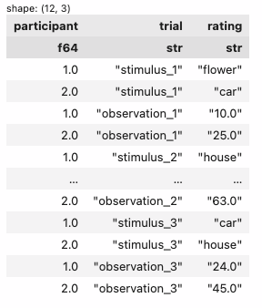
# Your code here

NoteSolution

step1 = reshape.unpivot(
    on=cs.exclude('participant'),
    index='participant',
    variable_name='trial',
    value_name='rating'
)
step1

shape: (12, 3)

participant	trial	rating
f64	str	str
1.0	"stimulus_1"	"flower"
2.0	"stimulus_1"	"car"
1.0	"observation_1"	"10.0"
2.0	"observation_1"	"25.0"
1.0	"stimulus_2"	"house"
…	…	…
2.0	"observation_2"	"63.0"
1.0	"stimulus_3"	"car"
2.0	"stimulus_3"	"house"
1.0	"observation_3"	"24.0"
2.0	"observation_3"	"45.0"

2. split the variable_name column from the previous step (I called it trial) into 2 new columns by _ (which I called index and order)

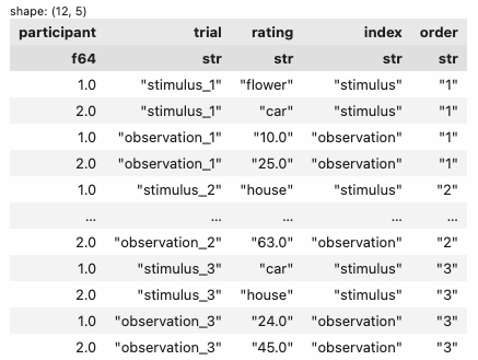
# Your code here

NoteSolution

step2 = step1.with_columns(
    col('trial').str.split_exact('_', 1).struct.rename_fields(['index', 'order']).struct.unnest()
)
step2

shape: (12, 5)

participant	trial	rating	index	order
f64	str	str	str	str
1.0	"stimulus_1"	"flower"	"stimulus"	"1"
2.0	"stimulus_1"	"car"	"stimulus"	"1"
1.0	"observation_1"	"10.0"	"observation"	"1"
2.0	"observation_1"	"25.0"	"observation"	"1"
1.0	"stimulus_2"	"house"	"stimulus"	"2"
…	…	…	…	…
2.0	"observation_2"	"63.0"	"observation"	"2"
1.0	"stimulus_3"	"car"	"stimulus"	"3"
2.0	"stimulus_3"	"house"	"stimulus"	"3"
1.0	"observation_3"	"24.0"	"observation"	"3"
2.0	"observation_3"	"45.0"	"observation"	"3"

3. select only the columns: participant, 2 you created (I called mine index and order), and the value_name column from the first step (I called it rating)

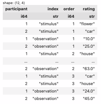
# Your code here

NoteSolution

step3 = step2.select(col('participant', 'index', 'order', 'rating'))
step3

shape: (12, 4)

participant	index	order	rating
f64	str	str	str
1.0	"stimulus"	"1"	"flower"
2.0	"stimulus"	"1"	"car"
1.0	"observation"	"1"	"10.0"
2.0	"observation"	"1"	"25.0"
1.0	"stimulus"	"2"	"house"
…	…	…	…
2.0	"observation"	"2"	"63.0"
1.0	"stimulus"	"3"	"car"
2.0	"stimulus"	"3"	"house"
1.0	"observation"	"3"	"24.0"
2.0	"observation"	"3"	"45.0"

4. pivot long -> wide to break-out the value_name column (I called it rating) into multiple columns

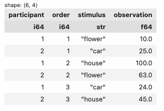
# Your code here

NoteSolution

step4 = step3.pivot(
    on='index',
    index=['participant', 'order'],
    values='rating',
    aggregate_function=None
)
step4

shape: (6, 4)

participant	order	stimulus	observation
f64	str	str	str
1.0	"1"	"flower"	"10.0"
2.0	"1"	"car"	"25.0"
1.0	"2"	"house"	"100.0"
2.0	"2"	"flower"	"63.0"
1.0	"3"	"car"	"24.0"
2.0	"3"	"house"	"45.0"

---

Appendix

Additional Resources

Here a few additional resources that might be helpful on your journey:

• Polars official intro tutorial
• More Comprehensive intro to Polars
• TidyData analysis in Polars
• Polars patterns vs R’s dplyr