Categorical Predictors & Coding Schemes

Author

Eshin Jolly

Code

import polars as pl
from polars import col
import seaborn as sns
from bossanova import model

In the previous notebook we added a 2-level categorical predictor (Student: Yes / No) using treatment coding. That was straightforward — one dummy variable, one reference group, done.

But what happens when a predictor has 3 or more levels? And does it matter how we code those levels into numbers?

Spoiler: the individual parameter estimates do change with different coding schemes, but there’s a test that gives the same answer no matter what. Understanding when and why is the key lesson of this notebook.

By the end you’ll know how to:

Encode a 3+ level categorical predictor as multiple dummy variables
Apply three coding schemes: treatment, sum, and polynomial
Inspect the design matrix to see exactly what each scheme does
Use .jointtest() to ask “does this predictor matter at all?” — and understand why the answer is invariant to coding
Distinguish between the joint test (omnibus) and individual parameter questions
Combine multiple categorical predictors (additive & interaction)

Code

credit = pl.read_csv("./data/credit.csv")
credit.head()

shape: (5, 12)

Index	Income	Limit	Rating	Cards	Age	Education	Gender	Student	Married	Ethnicity	Balance
i64	f64	i64	i64	i64	i64	i64	str	str	str	str	i64
1	14.891	3606	283	2	34	11	"Male"	"No"	"Yes"	"Caucasian"	333
2	106.025	6645	483	3	82	15	"Female"	"Yes"	"Yes"	"Asian"	903
3	104.593	7075	514	4	71	11	"Male"	"No"	"No"	"Asian"	580
4	148.924	9504	681	3	36	11	"Female"	"No"	"No"	"Asian"	964
5	55.882	4897	357	2	68	16	"Male"	"No"	"Yes"	"Caucasian"	331

Quick reminder of the variables we’ll focus on today:

Variable	Description	Type
Balance	Average credit card debt ($)	Continuous
Ethnicity	African American / Asian / Caucasian	Categorical (3 levels)
Gender	Male / Female	Categorical (2 levels)
Student	Yes / No	Categorical (2 levels)
Married	Yes / No	Categorical (2 levels)

Three-Level Categorical: The Default

In the previous notebook we modeled Student (2 levels) — that required 1 dummy column ($k - 1 = 2 - 1 = 1$).

Now let’s look at Ethnicity, which has 3 levels: African American, Asian, Caucasian. That means we need $k - 1 = 2$ dummy columns.

By default the reference level is the first alphabetical level of the factor. In this case African American:

\[ Balance_i = \beta_0 + \beta_1 \cdot Ethnicity[Asian]_i + \beta_2 \cdot Ethnicity[Caucasian]_i \]

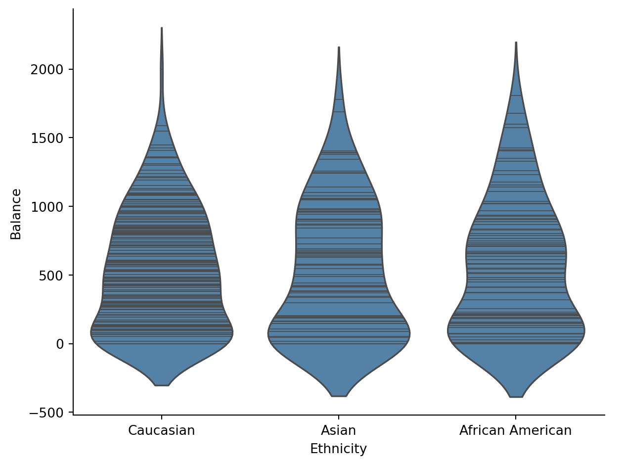
Let’s visualize first:

Code

sns.catplot(
    data=credit.to_pandas(),
    x="Ethnicity",
    y="Balance",
    kind="violin",
    inner="stick",
    height=5,
    aspect=1.3,
    color="steelblue",
)

Now let’s take a look at the design matrix:

Code

m_eth = model("Balance ~ Ethnicity", credit)
m_eth.plot_design()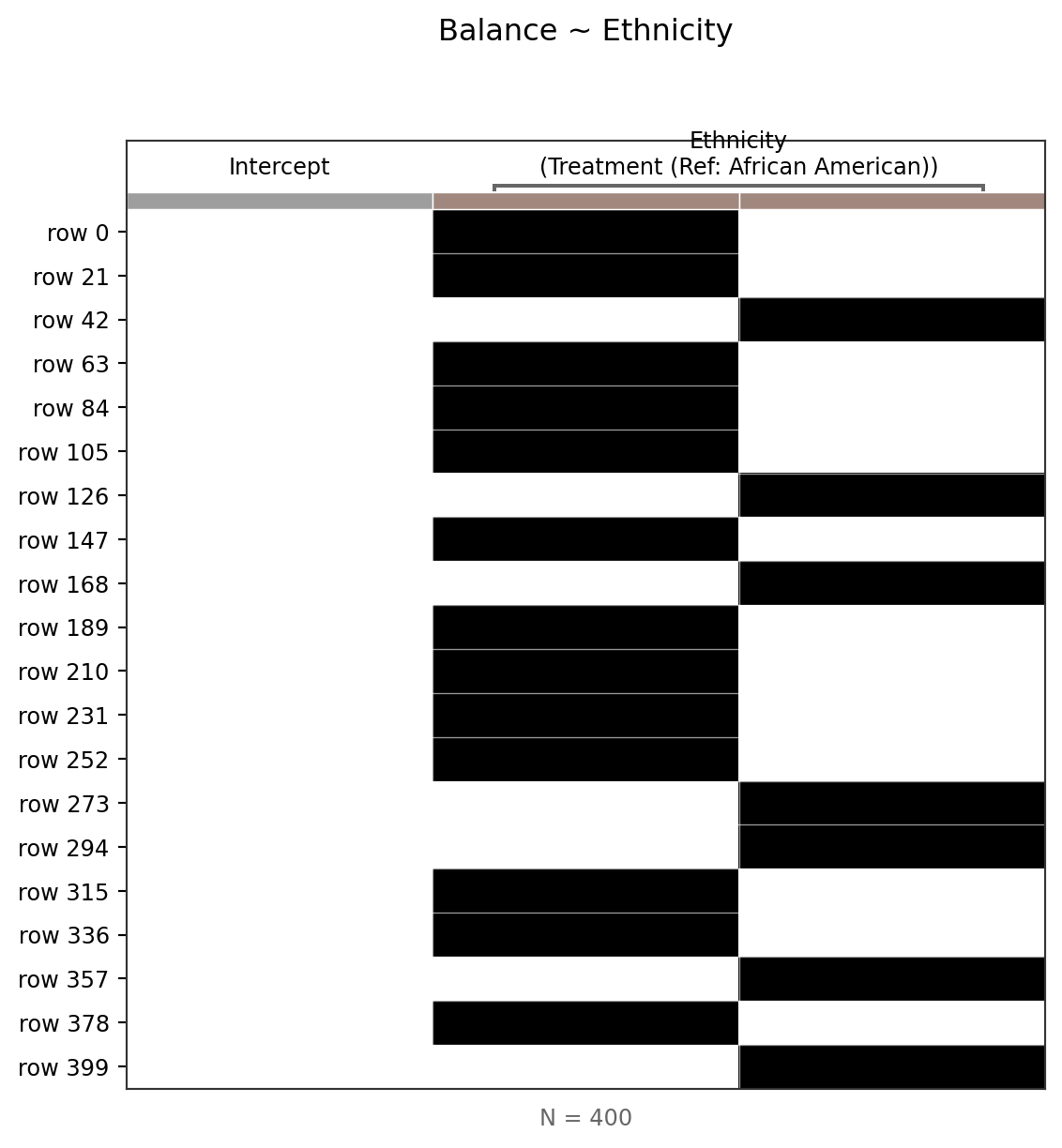

Code

m_eth.designmat.head()

shape: (5, 3)

Intercept	Ethnicity[Asian]	Ethnicity[Caucasian]
f64	f64	f64
1.0	0.0	1.0
1.0	1.0	0.0
1.0	1.0	0.0
1.0	1.0	0.0
1.0	0.0	1.0

Let’s try to understand what the default encoding is doing here by just grabbing the unique rows that correspond to each unique factor level of Ethnicity:

Code

# Sort just to make it easier to discuss
m_eth.designmat.unique().sort(by='Ethnicity[Caucasian]')

shape: (3, 3)

Intercept	Ethnicity[Asian]	Ethnicity[Caucasian]
f64	f64	f64
1.0	1.0	0.0
1.0	0.0	0.0
1.0	0.0	1.0

Here’s how we can read this:

Each row corresponds to one unique possible factor level. From top to bottom:
- [1 0 0]: African American
- [1 1 0]: Asian
- [1 0 1]: Caucasian
Each column corresponds to what that model parameter represents. From left to right:
- Intercept: mean of African American
- Ethnicity[Asian]: difference between Asian - African American
- Ethnicity[Caucasian]: difference between Caucasian - African American

And in GLM terms:

The reference level is chosen alphabetically → African American
$\beta_0$ (Intercept) = mean Balance for African Americans
$\beta_1$ (Ethnicity[Asian]) = Asian mean $-$ African American mean
$\beta_2$ (Ethnicity[Caucasian]) = Caucasian mean $-$ African American mean

With 3 levels we get $k - 1 = 2$ dummy columns. The reference group doesn’t need its own column — it’s captured by the Intercept.

Code

# Group Means:
group_means = (
    credit
    .group_by("Ethnicity")
    .agg(col("Balance").mean().alias("mean_balance"))
    .sort("Ethnicity")
)
group_means

shape: (3, 2)

Ethnicity	mean_balance
str	f64
"African American"	531.0
"Asian"	512.313725
"Caucasian"	518.497487

Code

# Parameter estimates
m_eth.fit().params

shape: (3, 2)

term	estimate
str	f64
"Intercept"	531.0
"Ethnicity[Asian]"	-18.69
"Ethnicity[Caucasian]"	-12.5

Three Coding Schemes

Above we met the default way the GLM handles categorical predictors (switches) and we learned that this called treatment coding in class. But this is just one way to convert categories into numbers.

Different coding schemes change what the Intercept and slopes mean, but — as we’ll see — they don’t change the model’s overall fit or predictions.

Let’s compare three schemes side-by-side.

1. Treatment Coding (default)

We’ve already seen this one:

Property	Value
Intercept	Mean of the reference group
Each slope	Difference from reference group
Design matrix	0/1 pattern (reference = all zeros)
Best when	There’s a natural reference group (e.g., control condition)

Code

# Recap: treatment coding params (already fit above)
m_eth.params

shape: (3, 2)

term	estimate
str	f64
"Intercept"	531.0
"Ethnicity[Asian]"	-18.69
"Ethnicity[Caucasian]"	-12.5

But we can control which group is the reference group directly in the model formula using treatment() and fitting again:

Code

# bossanova methods can be chained like polars!
(
    model("Balance ~ treatment(Ethnicity, ref='Caucasian')", credit) # contrasts in-formula
    .fit() # fit model
    .params # inspect params
)

shape: (3, 2)

term	estimate
str	f64
"Intercept"	518.5
"Ethnicity[African American]"	12.5
"Ethnicity[Asian]"	-6.184

Notice how the Intercept now reflect the mean of the Caucasian group. Like other software bossanova will automatically calculate the remaining codes for the other factor levels, but loses their names (because you can specify very complicated codes!).

Code

# Reverse alphabetical sort using the negative list slicing trick!
group_means[::-1]

shape: (3, 2)

Ethnicity	mean_balance
str	f64
"Caucasian"	518.497487
"Asian"	512.313725
"African American"	531.0

Your Turn

Can you figure out what the other parameters represent? Make a figure in seaborn to help you visualize the data and check

hint: we’ve simply moved things around so the “frame-of-reference” is the Caucasian group

Code

# Your code here

2. Sum (Deviation) Coding

In class we discussed how we can mean center continuous (slider) variables in our model to help with interpretability (and multi-collinearity). You can think of sum (deviation) coding as approximately equivalent for categorical (switch) variables.

Sum coding changes what the Intercept and slopes represent:

Property	Value
Intercept	Grand mean (unweighted mean of group means)
Each slope	Deviation of that group from the grand mean
Design matrix	-1 / 0 / 1 pattern (last group = all -1s)
Best when	No natural reference; you want each group compared to the overall average

The key property: each column in the design matrix sums to zero across levels — hence “sum” coding.

Code

m_sum = model("Balance ~ sum(Ethnicity)", credit)
m_sum.plot_design()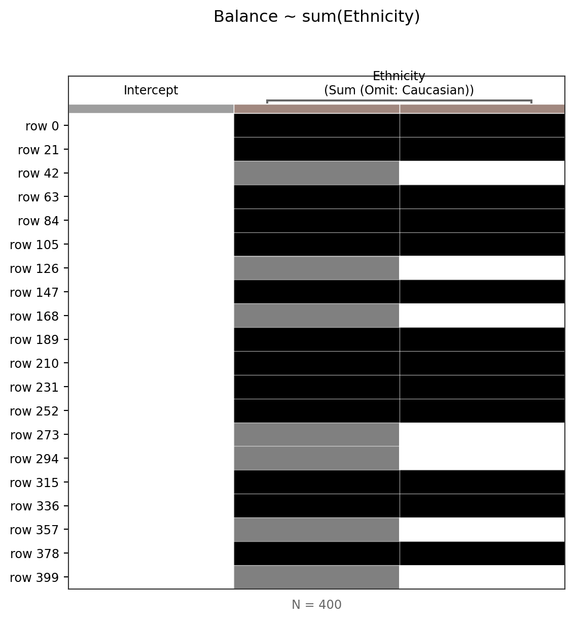

Code

m_sum.designmat.unique()

shape: (3, 3)

Intercept	Ethnicity[African American]	Ethnicity[Asian]
f64	f64	f64
1.0	0.0	1.0
1.0	1.0	0.0
1.0	-1.0	-1.0

Notice the -1 / 0 / 1 pattern in the design matrix. The last level alphabetically (Caucasian) gets coded as -1 on both columns — it’s the “omitted” group whose deviation can be recovered as the negative sum of the other deviations.

You can interpret this encoding scheme as having the same effect that mean centering has on continuous (slider) predictors. It removes collinearity, but in the case of factor levels makes things harder to interpet, with the benefit being that it also “balances out” any differences in group size that you may have when you make comparisons.

Why columns sum to zero

In sum coding, the contrast columns are designed so that the Intercept estimates the grand mean — the unweighted average across all group means. Each slope then measures how far a group deviates from that average.

This is the coding scheme most naturally connected to ANOVA-style thinking, where we ask “how do groups differ from the overall average?” while accounting for imbalances in group-sizes.

Code

# Verify: Intercept should be the grand mean (unweighted mean of group means)
grand_mean = group_means.select(col("mean_balance").mean())
grand_mean

shape: (1, 1)

mean_balance
f64
520.603738

Code

m_sum.fit().params

shape: (3, 2)

term	estimate
str	f64
"Intercept"	520.6
"Ethnicity[African American]"	10.4
"Ethnicity[Asian]"	-8.29

Your Turn

Like before, see if you can figure out what the other two parameters represent in terms of group-means. It’s tricky! And you’ll need to “mix” groups together

Code

# Your code here

3. Polynomial Coding

Polynomial coding is extremely useful whenever your factor levels (or hypotheses about them) are ordered. For example: “is there a linear trend across groups?”

Property	Value
Intercept	Grand mean
Slopes	Linear trend, quadratic trend, etc.
Design matrix	Orthogonal polynomial contrasts
Best when	Levels have a natural ordering (e.g., Low / Medium / High)

Let’s see what happens when we apply it to Ethnicity — even though Ethnicity has no natural ordering.

For Ethnicity, the order is just alphabetical — there’s no reason “African American → Asian → Caucasian” should be treated as a progression, so the “linear” and “quadratic” trends are not particularly informative in this example, but you can imagine a study design or dataset where they might be (e.g. pain severity, ses, etc).

Code

m_poly = model("Balance ~ poly(Ethnicity)", credit)
m_poly.plot_design()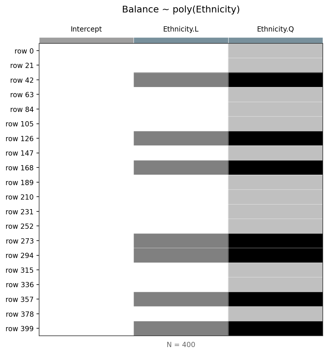

Code

m_poly.designmat.unique()

shape: (3, 3)

Intercept	Ethnicity.L	Ethnicity.Q
f64	f64	f64
1.0	-0.707107	0.408248
1.0	0.707107	0.408248
1.0	-1.6940e-17	-0.816497

The design matrix shows orthogonal contrast weights. The first parameter captures a “linear” trend across levels, and the second captures a “quadratic” (U-shaped) trend. Orthogonal means “statistical independent” (in a linear sense), so we’ve de-correlated these predictors as much as possible.

For example check out the correlation between polynomial encoding:

Code

m_poly.plot_vif()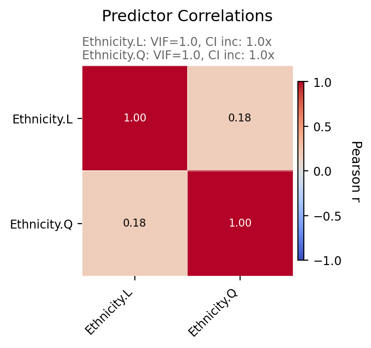

Vs sum coding:

Code

m_sum.plot_vif()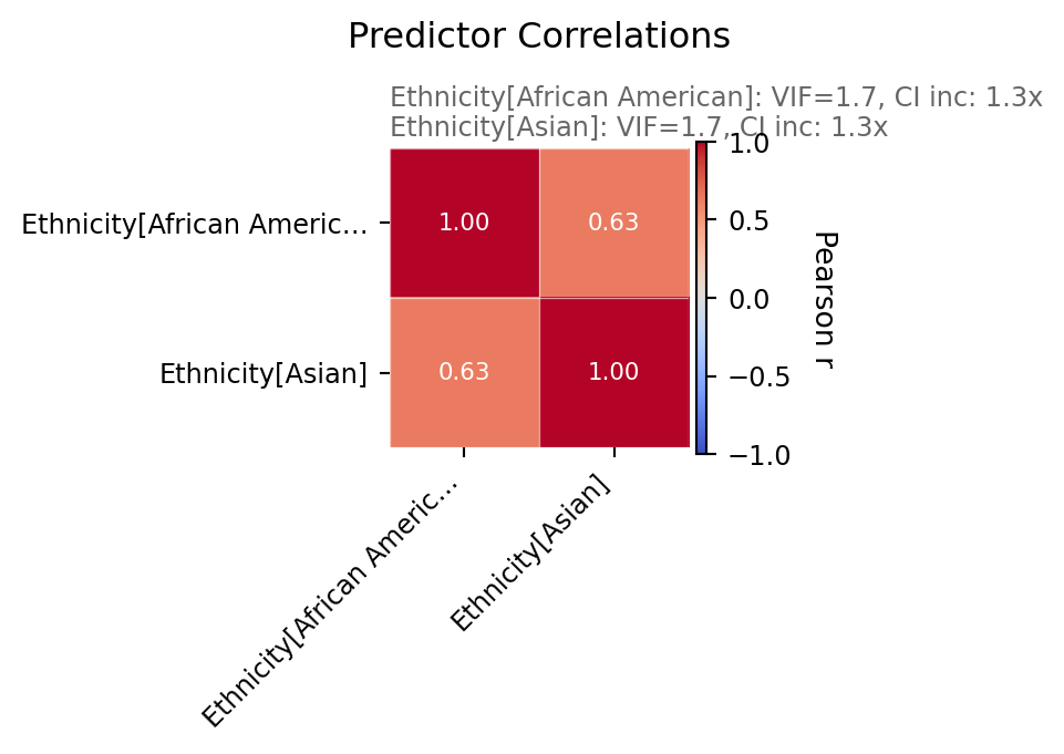

But critically notice that the model’s predictions do not change!

We’re just mixing things around but not fundamentally changing anything about the GLM’s behavior!

Code

# Each model's predictions (re-fit so this cell is self-contained)
all_fits = pl.DataFrame({"Treatment": m_eth.fit().data['fitted'], "Sum": m_sum.fit().data['fitted'], "Poly": m_poly.fit().data["fitted"]})

# Make a correlation matrix
ax = sns.heatmap(all_fits.corr().to_pandas(), vmin=-1, vmax=1, cmap='coolwarm', linewidths=1, annot=True, yticklabels=all_fits.columns)
ax.set_title("Correlation Matrix of Model Predictions")

Text(0.5, 1.0, 'Correlation Matrix of Model Predictions')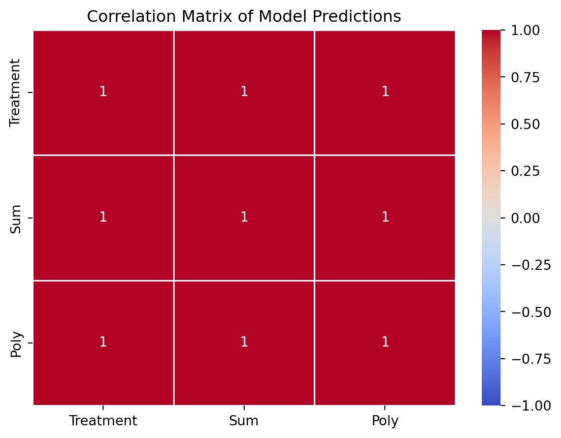

Coding Schemes Summary

	Treatment	Sum	Polynomial
Intercept	Reference group mean	Grand mean	Grand mean
Slopes	Differences from reference	Deviations from grand mean	Linear, quadratic, … trends
Design matrix	0 / 1	-1 / 0 / 1	Orthogonal weights
Use when	Natural reference group	No natural reference, ANOVA-style	Ordered levels
Predictions	Same	Same	Same
$R^2$	Same	Same	Same

Joint (Omnibus/ANOVA tests) & Model Comparison

Here’s the big idea to connect a few pieces together:

We have a factor with 3 levels, but the exact estimates we calculate depend on our coding scheme
We’re just interested in whether Ethnicity matters overall for predicting credit-card balance
So how can we do this? Model comparison

Code

from bossanova import compare

Code

# Compact model: no Ethnicity (intercept only)
m_compact = model("Balance ~ 1", credit).fit()

# compare() should give the same F and p-value as jointtest()
compare(m_compact, m_eth)

shape: (2, 8)

model	PRE	F	rss	ss	df	df_resid	p_value
str	f64	f64	f64	f64	f64	f64	f64
"Balance ~ 1"	null	null	8.434e7	null	null	399.0	null
"Balance ~ Ethnicity"	0.000219	0.04344	8.432e7	18450.0	2.0	397.0	0.9575

Now run the next code cell and check-out the output:

Code

m_eth.jointtest()

shape: (1, 5)

term	df1	df2	f_ratio	p_value
str	i64	f64	f64	f64
"Ethnicity"	2	397.0	0.043443	0.957492

This is the most important idea in this notebook: ANOVA = Nested Model Comparison

The .jointtest() method is how bossanova computes a what we call traditional Analysis of Variance (ANOVA). However, we’ve named it more informatively based on what it actually does, just like the same function in R’s emmeans package.

An omnibus/F/jointtest, tests all parameters that reflect a factor variable simulataneously (hence the name). But what does “test simultaneously mean?”

It’s just nested model comparison between a compact model without the term, and an augmented model including the term. The F-ratio tells us the uncertainty we should have in our PRE when this term is included in the model - how much better does it predict credit card balance?

Critically, our coding scheme does not effect the joint-test!

We’ll explain more in class, but what jointtest is doing behind-the-scenes is what Psychologists (almost exclusively) call a “Type-III Sum-of-Squares” test.

This is consistent with modern tools in R like the tidyverse that automatically handle this for you.

However, if you’re manually doing this with other tools in Python or in R (e.g. the aov() or anova() functions) you first must use either sum or polynomial encoding to get valid traditional ANOVA/jointtest results!

This is just a (pointless) statistical relic that bossanova just does the “right thing” for you when you ask for a jointtest.

Code

# Sum coding
m_sum.jointtest()

shape: (1, 5)

term	df1	df2	f_ratio	p_value
str	i64	f64	f64	f64
"Ethnicity"	2	397.0	0.043443	0.957492

Code

# Polynomial coding
m_poly.jointtest()

shape: (2, 5)

term	df1	df2	f_ratio	p_value
str	i64	f64	f64	f64
"Ethnicity.L"	1	397.0	0.048654	0.825535
"Ethnicity.Q"	1	397.0	0.053588	0.817052

The F-statistic and p-value from compare() match .jointtest() exactly. They’re asking the same question: “Is Ethnicity worth including in the model?”

Joint test vs individual parameters — when to use which

Question Tool Coding-dependent?

“Does Ethnicity matter at all?” .jointtest() or compare() No — always the same answer

“How does Asian differ from African American?” .params with treatment coding Yes — depends on reference level

“How does each group deviate from the grand mean?” .params with sum coding Yes — depends on coding scheme

Think of it this way: the joint test asks whether the predictor is worth including, while the individual parameters tell you the specific pattern — and the pattern’s description depends on how you coded the levels.

Question	Tool	Coding-dependent?
“Does Ethnicity matter at all?”	`.jointtest()` or `compare()`	No — always the same answer
“How does Asian differ from African American?”	`.params` with treatment coding	Yes — depends on reference level
“How does each group deviate from the grand mean?”	`.params` with sum coding	Yes — depends on coding scheme

Two Factor Models

Let’s increase the complexity a bit and include Student (which we’ve previously seen) as another variable. Remember it has 2 levels (Yes/No).

We’ll start with the default (treatment coding):

Code

m_add = model("Balance ~ Ethnicity + Student", credit)
m_add.plot_design()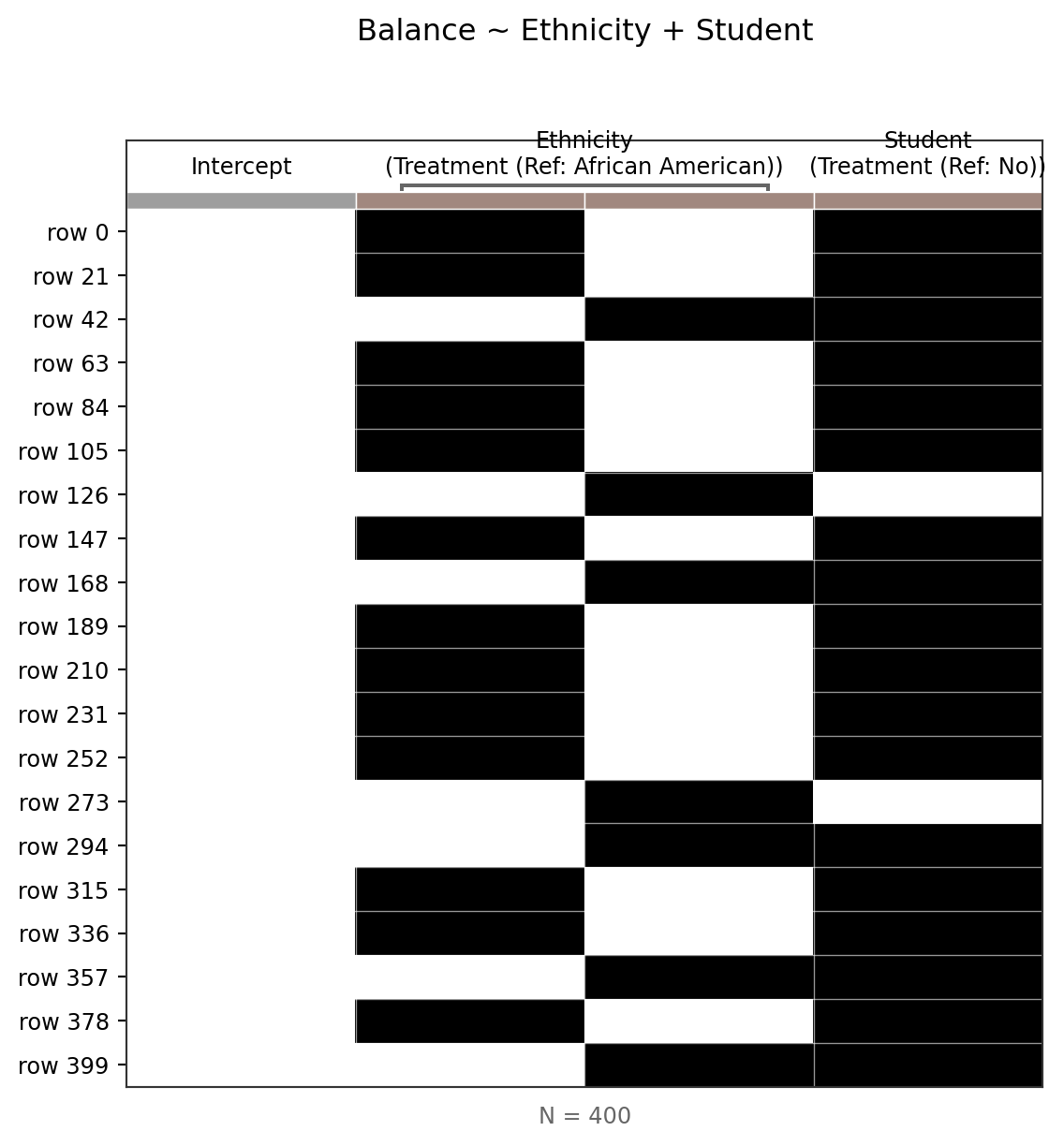

Code

m_add.designmat.unique()

shape: (6, 4)

Intercept	Ethnicity[Asian]	Ethnicity[Caucasian]	Student[Yes]
f64	f64	f64	f64
1.0	0.0	1.0	0.0
1.0	0.0	0.0	1.0
1.0	0.0	1.0	1.0
1.0	1.0	0.0	0.0
1.0	1.0	0.0	1.0
1.0	0.0	0.0	0.0

Notice now how there are 6 unique combinations required to capture all of our factor level combinations:

Ethnicity: 3 levels, k = 2
Student: 2 levels, k = 1
2 + 1 = 3 columns to represent all possible differences
3 + 2 (+ 1) = 6 combinations to represent each unique difference

Code

m_add.fit().params

shape: (4, 2)

term	estimate
str	f64
"Intercept"	490.8
"Ethnicity[Asian]"	-29.22
"Ethnicity[Caucasian]"	-6.297
"Student[Yes]"	398.2

Your turn

See if you can figure out what these parameter estimates represent?

Code

# Your code here

Let’s take it a step further and include an interaction:

Code

m_int = model("Balance ~ Ethnicity * Student", credit)
m_int.plot_design()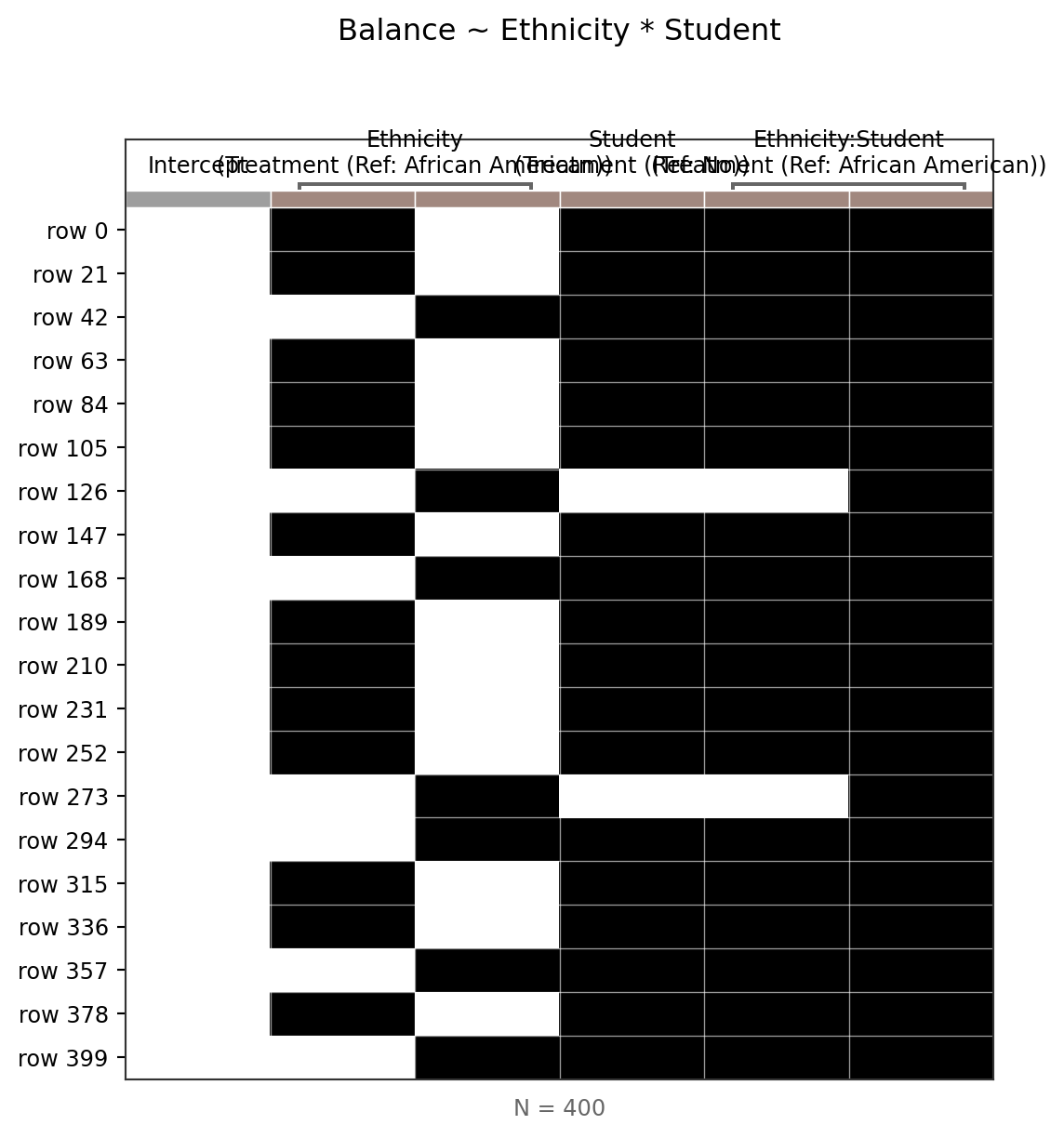

Code

m_int.designmat.unique()

shape: (6, 6)

Intercept	Ethnicity[Asian]	Ethnicity[Caucasian]	Student[Yes]	Ethnicity[Asian]:Student[Yes]	Ethnicity[Caucasian]:Student[Yes]
f64	f64	f64	f64	f64	f64
1.0	1.0	0.0	0.0	0.0	0.0
1.0	1.0	0.0	1.0	1.0	0.0
1.0	0.0	1.0	0.0	0.0	0.0
1.0	0.0	0.0	1.0	0.0	0.0
1.0	0.0	1.0	1.0	0.0	1.0
1.0	0.0	0.0	0.0	0.0	0.0

Your turn

Call .fit() and then inspect .params and try to understand what each parameter reflects in terms of factor level differences.

It’ll be helpful to use polars to aggregate the groups first and verify

Code

# You code here

Now let’s run a jointtest (traditional ANOVA):

Code

m_int.jointtest()

shape: (3, 5)

term	df1	df2	f_ratio	p_value
str	i64	f64	f64	f64
"Ethnicity"	2	394.0	0.818464	0.441857
"Student"	1	394.0	30.881767	5.0597e-8
"Ethnicity:Student"	2	394.0	1.513414	0.221434

Row 1 represents the “main effect” of Ethnicity
Row 2 represents the “main effect” of Student
Row 3 represents their interaction

Let’s try to understand what’s happening by seeing this as the equivalent set of model comparisons starting with the interaction.

To test if the interaction is worth it we need create a compact model thats the same in everyway except the interaction:

That’s just our Balance ~ Ethnicity + Student model from earlier!

Code

compare(m_add, m_int)

shape: (2, 8)

model	PRE	F	rss	ss	df	df_resid	p_value
str	f64	f64	f64	f64	f64	f64	f64
"Balance ~ Ethnicity + Student"	null	null	7.863e7	null	null	396.0	null
"Balance ~ Ethnicity * Student"	0.007624	1.513	7.803e7	599500.0	2.0	394.0	0.2214

Notice how the F-ration and p-values are identitical to the last row of the jointtest

Now to test “main effects” we need to remove 1 variable at a time, while keeping in mind they contribute to the interaction. It’s helpful to keep in mind that this formula:

Balance ~ Ethnicity * Student is really:

Balance ~ Ethnicity + Student + Ethnicity:Student

So we need to create 2 more nested models:

Code

# Drop Ethnicity (keep interaction!)
drop_eth = model("Balance ~ Student + Ethnicity:Student", credit).fit()

# Drop Student (keep interaction!)
drop_student = model("Balance ~ Ethnicity + Ethnicity:Student", credit).fit()

Code

# Main effect of Ethnicity
compare(drop_eth, m_int)

shape: (2, 8)

model	PRE	F	rss	ss	df	df_resid	p_value
str	f64	f64	f64	f64	f64	f64	f64
"Balance ~ Student + Ethnicity:…	null	null	7.819e7	null	null	396.0	null
"Balance ~ Ethnicity * Student"	0.002005	0.3958	7.803e7	156800.0	2.0	394.0	0.6734

Code

# Main effect of Student
compare(drop_student, m_int)

shape: (2, 8)

model	PRE	F	rss	ss	df	df_resid	p_value
str	f64	f64	f64	f64	f64	f64	f64
"Balance ~ Ethnicity + Ethnicit…	null	null	8.026e7	null	null	395.0	null
"Balance ~ Ethnicity * Student"	0.02777	11.25	7.803e7	2.229e6	1.0	394.0	0.0008723

Code

# Just to compare
m_int.jointtest()

shape: (3, 5)

term	df1	df2	f_ratio	p_value
str	i64	f64	f64	f64
"Ethnicity"	2	394.0	0.818464	0.441857
"Student"	1	394.0	30.881767	5.0597e-8
"Ethnicity:Student"	2	394.0	1.513414	0.221434

Your Turn

Use the cells below to practice. Some ideas:

Fit Balance ~ Gender and Balance ~ Married — check the joint tests and params
Try changing the reference level for treatment coding
Verify that the joint test is still the same with a different reference level
Fit a large model with all categorical predictors and inspect its .jointtest(): Balance ~ Ethnicity * Student * Gender
Use compare() and any new nested mdoels you need to create to match the output of each main-effect and interaction

Tip: If you’re confused make some plots to help you out!

Code

credit.head()

shape: (5, 12)

Index	Income	Limit	Rating	Cards	Age	Education	Gender	Student	Married	Ethnicity	Balance
i64	f64	i64	i64	i64	i64	i64	str	str	str	str	i64
1	14.891	3606	283	2	34	11	"Male"	"No"	"Yes"	"Caucasian"	333
2	106.025	6645	483	3	82	15	"Female"	"Yes"	"Yes"	"Asian"	903
3	104.593	7075	514	4	71	11	"Male"	"No"	"No"	"Asian"	580
4	148.924	9504	681	3	36	11	"Female"	"No"	"No"	"Asian"	964
5	55.882	4897	357	2	68	16	"Male"	"No"	"Yes"	"Caucasian"	331

Code

# Your code here

Code

# Your code here

Code

# Your code here