Odds and Ends (stuff we didn’t get to)

Author

Eshin Jolly

Published

March 11, 2026

Code

import numpy as np
import polars as pl
import seaborn as sns
import matplotlib.pyplot as plt
from bossanova import model, load_dataset
from sklearn.datasets import load_diabetes, load_digits, load_iris, make_moons
from sklearn.linear_model import LinearRegression, Ridge, RidgeCV, Lasso, LassoCV
from sklearn.model_selection import (
    cross_val_score,
    LeaveOneGroupOut,
    TimeSeriesSplit,
)
from sklearn.preprocessing import StandardScaler
from sklearn.pipeline import make_pipeline
from sklearn.decomposition import PCA, FastICA, FactorAnalysis
from sklearn.svm import SVC
from sklearn.naive_bayes import GaussianNB

This notebook demos additional topics we did not get to cover in depth. For most of your statistical needs your first stop should be the sklearn library that we met once before in the course. This notebook demos many of the common topics you might want to apply to your own data

Cross-validation

Cross-validation estimates how well a model generalizes to unseen data. Instead of evaluating on the same data you trained on (which is overoptimistic), you repeatedly hold out a portion of data for testing and train on the rest. The most common variant is k-fold CV: split data into \(k\) equal parts, train on \(k-1\), test on the held-out fold, rotate through all \(k\) folds, and average.

\[ \text{CV}(k) = \frac{1}{k} \sum_{i=1}^{k} L\bigl(y_{\text{test}}^{(i)},\; \hat{f}^{(-i)}(X_{\text{test}}^{(i)})\bigr) \]

where \(\hat{f}^{(-i)}\) is the model trained on all folds except fold \(i\), and \(L\) is a loss function (e.g. MSE, R²).

Using `bossanova`

In bossanova, .infer(how="cv") runs k-fold CV and computes a PRE (Proportion Reduction in Error) for each predictor — how much worse does out-of-sample prediction get when you drop that term? This is the cross-validated analogue of the PRE you already know from compare().

Code

adv = load_dataset("advertising")

m_adv = model("sales ~ tv + radio + newspaper", adv).fit()
m_adv.infer(how="cv", k=5, seed=42)
m_adv.params

shape: (4, 4)

term	estimate	pre	pre_sd
str	f64	f64	f64
"Intercept"	2.939	0.0	0.0
"tv"	0.04576	0.651	0.1368
"radio"	0.1885	0.2846	0.104
"newspaper"	-0.001037	-0.000827	0.0006964

shape: (4, 4)

term	estimate	pre	pre_sd
str	f64	f64	f64
"Intercept"	2.939	0.0	0.0
"tv"	0.04576	0.651	0.1368
"radio"	0.1885	0.2846	0.104
"newspaper"	-0.001037	-0.000827	0.0006964

More generally using `sklearn`

Scikit Learn (sklearn) is the de-facto machine-learning library for Python. It also has fantastic tutorials and documentations to help you learn many additional concepts easily.

Once of those is a huge set of options for fully controllong how you do cross-validation. Common splitters include KFold (default), LeaveOneGroupOut (hold out entire clusters — critical for repeated measures), and TimeSeriesSplit (respects temporal ordering so you never train on the future).

While we didn’t cover it in detail, sklearn makes heavy use of the numpy library and expects any \(X\) or \(y\) to be a numpy array (1d or 2d vector or matrix):

Code

X_diabetes, y_diabetes = load_diabetes(return_X_y=True)

# Design matrix
X_diabetes.shape

(442, 10)

Code

y_diabetes.shape

(442,)

Code

# 1) Create the model
lr = LinearRegression()

# 2) Use cross-validator
scores = cross_val_score(lr, X_diabetes, y_diabetes, cv=5, scoring="r2")

print(f"5-fold R²: {scores.mean():.3f} ± {scores.std():.3f}")
print(f"Per-fold:  {np.round(scores, 3)}")

5-fold R²: 0.482 ± 0.049
Per-fold:  [0.43  0.523 0.483 0.426 0.55 ]

Scoring functions control what metric is computed on each fold. Common choices:

Scoring string	What it measures
`"r2"`	Proportion of variance explained (regression)
`"neg_mean_squared_error"`	Negative MSE (regression; negative so “higher is better”)
`"accuracy"`	Fraction correct (classification)
`"roc_auc"`	Area under ROC curve (classification)

Decomposition

sklearn also offers many methods for decomposition, when our model only has an \(X\) — there’s no outcome \(y\). These fall under the broader topic of unsupervised learning and work by factorizing the data matrix into lower-rank components. The goal is to find a small number of latent dimensions that capture most of the structure in high-dimensional data.

\[ X_{n \times p} \approx W_{n \times k} \cdot H_{k \times p} \]

where \(k \ll p\). Different methods impose different constraints on \(W\) and \(H\).

Principal Components Analysis (PCA)

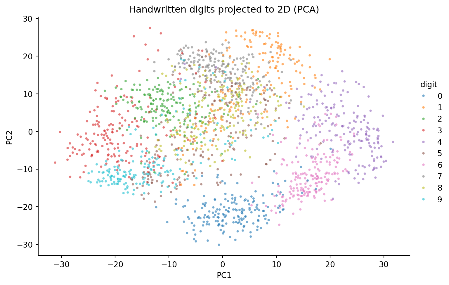
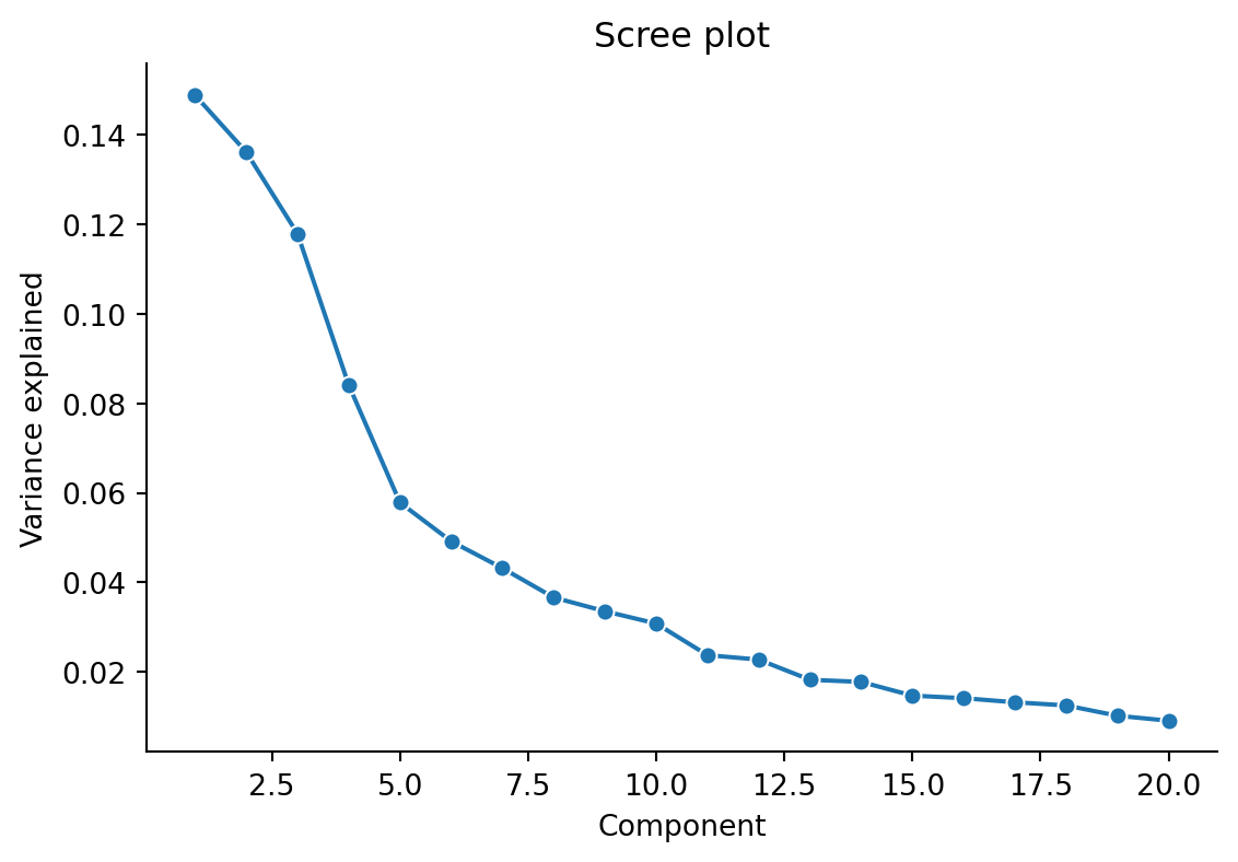
PCA finds orthogonal directions of maximum variance in the data. The first principal component captures the most variance, the second captures the most remaining variance (orthogonal to the first), and so on. Mathematically, PCA computes the eigendecomposition of the covariance matrix:

\[ \Sigma = \frac{1}{n} X^\top X = V \Lambda V^\top \]

where \(V\) are the eigenvectors (principal directions) and \(\Lambda\) are the eigenvalues (variance explained per component).

Code

# Dataset of handwritten digits as images
digits = load_digits()

# Create estimator
pca = PCA(n_components=2)

# Fit it and project data to PC space
X_pca = pca.fit_transform(digits.data)

Code

# Plot it
_pca_df = pl.DataFrame({
    "PC1": X_pca[:, 0],
    "PC2": X_pca[:, 1],
    "digit": [str(d) for d in digits.target],
})

sns.relplot(
    data=_pca_df.to_pandas(),
    x="PC1", y="PC2",
    hue="digit", palette="tab10",
    kind="scatter", s=10, alpha=0.6,
    height=5, aspect=1.5,
).set(title="Handwritten digits projected to 2D (PCA)")

Code

_pca_full = PCA().fit(load_digits().data)

_scree_df = pl.DataFrame({
    "component": list(range(1, 21)),
    "variance_explained": _pca_full.explained_variance_ratio_[:20].tolist(),
})

sns.relplot(
    data=_scree_df.to_pandas(),
    x="component", y="variance_explained",
    kind="line", marker="o",
    height=4, aspect=1.5,
).set(title="Scree plot", xlabel="Component", ylabel="Variance explained")

Factor Analysis

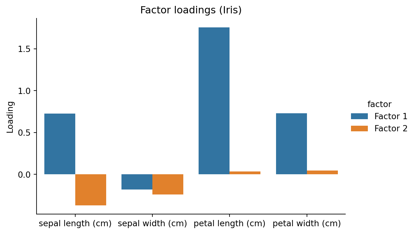
Factor Analysis assumes the observed variables are linear combinations of latent factors plus noise. Unlike PCA, it explicitly models measurement error and tries to recover interpretable latent constructs:

\[ X = \mu + L F + \epsilon, \qquad \epsilon \sim \mathcal{N}(0, \Psi) \]

where \(L\) is the loading matrix, \(F\) are the latent factors, and \(\Psi\) is a diagonal matrix of variable-specific noise. The key difference from PCA: Factor Analysis separates shared variance (factors) from unique variance (noise).

Code

iris = load_iris()

fa = FactorAnalysis(n_components=2, random_state=42)
fa.fit(iris.data)

# Build long-format loadings DataFrame
_loadings_df = pl.DataFrame({
    "feature": iris.feature_names * 2,
    "factor": ["Factor 1"] * 4 + ["Factor 2"] * 4,
    "loading": fa.components_.T[:, 0].tolist() + fa.components_.T[:, 1].tolist(),
})

sns.catplot(
    data=_loadings_df.to_pandas(),
    x="feature", y="loading", hue="factor",
    kind="bar", height=4, aspect=1.5,
).set(title="Factor loadings (Iris)", xlabel="", ylabel="Loading")

FactorAnalysis(n_components=2, random_state=42)

In a Jupyter environment, please rerun this cell to show the HTML representation or trust the notebook.
On GitHub, the HTML representation is unable to render, please try loading this page with nbviewer.org.

FactorAnalysis

?Documentation for FactorAnalysisiFitted

Parameters

	n_components n_components: int, default=None Dimensionality of latent space, the number of components of ``X`` that are obtained after ``transform``. If None, n_components is set to the number of features.	2
	random_state random_state: int or RandomState instance, default=0 Only used when ``svd_method`` equals 'randomized'. Pass an int for reproducible results across multiple function calls. See :term:`Glossary <random_state>`.	42
	tol tol: float, default=1e-2 Stopping tolerance for log-likelihood increase.	0.01
	copy copy: bool, default=True Whether to make a copy of X. If ``False``, the input X gets overwritten during fitting.	True
	max_iter max_iter: int, default=1000 Maximum number of iterations.	1000
	noise_variance_init noise_variance_init: array-like of shape (n_features,), default=None The initial guess of the noise variance for each feature. If None, it defaults to np.ones(n_features).	None
	svd_method svd_method: {'lapack', 'randomized'}, default='randomized' Which SVD method to use. If 'lapack' use standard SVD from scipy.linalg, if 'randomized' use fast ``randomized_svd`` function. Defaults to 'randomized'. For most applications 'randomized' will be sufficiently precise while providing significant speed gains. Accuracy can also be improved by setting higher values for `iterated_power`. If this is not sufficient, for maximum precision you should choose 'lapack'.	'randomized'
	iterated_power iterated_power: int, default=3 Number of iterations for the power method. 3 by default. Only used if ``svd_method`` equals 'randomized'.	3
	rotation rotation: {'varimax', 'quartimax'}, default=None If not None, apply the indicated rotation. Currently, varimax and quartimax are implemented. See `"The varimax criterion for analytic rotation in factor analysis" <https://link.springer.com/article/10.1007%2FBF02289233>`_ H. F. Kaiser, 1958. .. versionadded:: 0.24	None

Fitted attributes

Name	Type	Value
components_ components_: ndarray of shape (n_components, n_features) Components with maximum variance.	ndarray[float64](2, 4)	[[ 0.73,-0.18, 1.76, 0.73], [-0.37,-0.24, 0.04, 0.05]]
loglike_ loglike_: list of shape (n_iterations,) The log likelihood at each iteration.	list	[np.float64(-709.8923338622799), np.float64(-529.31618866758), np.float64(-4...5759820781625), np.float64(-4...8163431043125), ...]
mean_ mean_: ndarray of shape (n_features,) Per-feature empirical mean, estimated from the training set.	ndarray[float64](4,)	[5.84,3.06,3.76,1.2 ]
n_features_in_ n_features_in_: int Number of features seen during :term:`fit`. .. versionadded:: 0.24	int	4
n_iter_ n_iter_: int Number of iterations run.	int	121
noise_variance_ noise_variance_: ndarray of shape (n_features,) The estimated noise variance for each feature.	ndarray[float64](4,)	[0.02,0.1 ,0. ,0.04]

2 features

factoranalysis0
factoranalysis1

Independent Components Analysis (ICA)

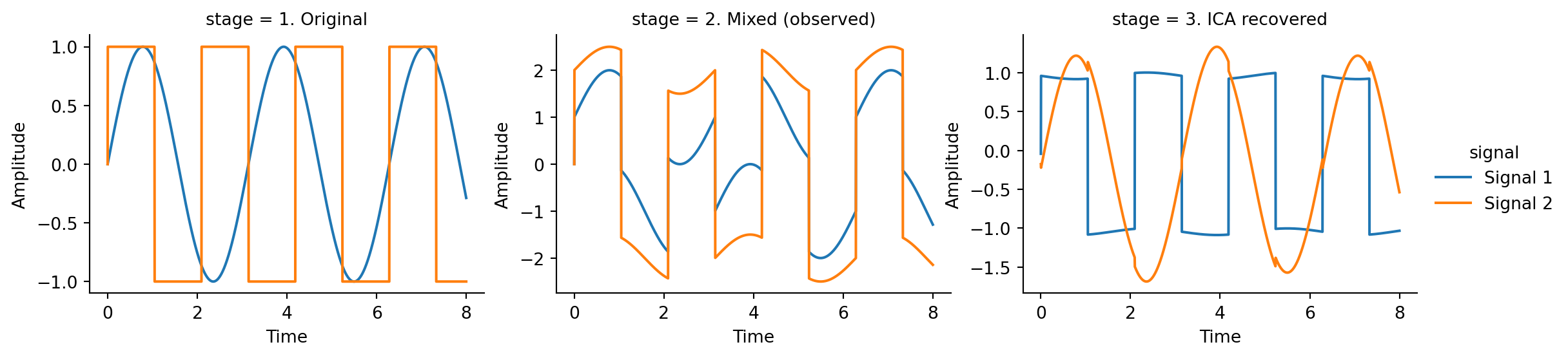
ICA finds components that are statistically independent (not just uncorrelated). The classic application is the “cocktail party problem”: separating mixed audio signals back into their original sources. ICA assumes the observed data are linear mixtures of independent non-Gaussian sources:

\[ X = A \cdot S \qquad \Rightarrow \qquad S = W \cdot X \]

where \(A\) is the unknown mixing matrix and \(W = A^{-1}\) is the unmixing matrix that ICA estimates.

Code

_t = np.linspace(0, 8, 2000)

# Original independent signals
_S_true = np.c_[np.sin(2 * _t), np.sign(np.sin(3 * _t))]

# Mix them with an unknown matrix
_X_mixed = _S_true @ np.array([[1, 1], [0.5, 2]]).T

# Recover with ICA
_S_recovered = FastICA(n_components=2, random_state=42).fit_transform(_X_mixed)

# Build long-format DataFrame for faceted plotting
_n = len(_t)
_ica_df = pl.DataFrame({
    "time": _t.tolist() * 6,
    "value": np.concatenate([
        _S_true[:, 0], _S_true[:, 1],
        _X_mixed[:, 0], _X_mixed[:, 1],
        _S_recovered[:, 0], _S_recovered[:, 1],
    ]).tolist(),
    "signal": (["Signal 1"] * _n + ["Signal 2"] * _n) * 3,
    "stage": (
        ["1. Original"] * (2 * _n)
        + ["2. Mixed (observed)"] * (2 * _n)
        + ["3. ICA recovered"] * (2 * _n)
    ),
})

sns.relplot(
    data=_ica_df.to_pandas(),
    x="time", y="value",
    hue="signal", col="stage",
    kind="line", height=3, aspect=1.3,
    facet_kws={"sharey": False},
).set(xlabel="Time", ylabel="Amplitude")

Regularization

When predictors are correlated or you have many features relative to observations, OLS estimates become unstable — small changes in data cause large swings in coefficients. Regularization adds a penalty term to the loss function that shrinks coefficients toward zero, trading a little bias for a lot less variance.

\[ \hat{\beta}_{\text{reg}} = \arg\min_\beta \left[ \sum_i (y_i - X_i \beta)^2 + \lambda \cdot \text{penalty}(\beta) \right] \]

The penalty strength \(\lambda\) controls the bias-variance tradeoff. We use cross-validation to pick the best \(\lambda\).

Ridge Regression

Ridge adds an L2 penalty — the sum of squared coefficients. This shrinks all coefficients toward zero but never sets them exactly to zero. It’s especially useful when predictors are correlated (multicollinearity):

\[ \hat{\beta}_{\text{ridge}} = \arg\min_\beta \left[ \|y - X\beta\|^2 + \lambda \sum_j \beta_j^2 \right] \]

Code

X_d, y_d = load_diabetes(return_X_y=True)

# Compare OLS vs Ridge at different penalty strengths
_alphas = [0, 0.01, 0.1, 1.0, 10.0, 100.0]
for _a in _alphas:
    _est = LinearRegression() if _a == 0 else Ridge(alpha=_a)
    _s = cross_val_score(_est, X_d, y_d, cv=5, scoring="r2")
    print(f"alpha={_a:<6}  R²={_s.mean():.3f} ± {_s.std():.3f}")

alpha=0       R²=0.482 ± 0.049
alpha=0.01    R²=0.481 ± 0.049
alpha=0.1     R²=0.480 ± 0.047
alpha=1.0     R²=0.410 ± 0.045
alpha=10.0    R²=0.138 ± 0.036
alpha=100.0   R²=-0.005 ± 0.036

Code

# Let CV pick the best alpha automatically
ridge_cv = RidgeCV(alphas=np.logspace(-3, 3, 50), scoring="r2")
ridge_cv.fit(X_d, y_d)
print(f"Best alpha: {ridge_cv.alpha_:.4f}")
print(f"Coefficients: {np.round(ridge_cv.coef_, 2)}")

RidgeCV(alphas=array([1.00000000e-03, 1.32571137e-03, 1.75751062e-03, 2.32995181e-03,
       3.08884360e-03, 4.09491506e-03, 5.42867544e-03, 7.19685673e-03,
       9.54095476e-03, 1.26485522e-02, 1.67683294e-02, 2.22299648e-02,
       2.94705170e-02, 3.90693994e-02, 5.17947468e-02, 6.86648845e-02,
       9.10298178e-02, 1.20679264e-01, 1.59985872e-01, 2.12095089e-01,
       2.81176870e-01, 3.72759372e-0...
       8.68511374e-01, 1.15139540e+00, 1.52641797e+00, 2.02358965e+00,
       2.68269580e+00, 3.55648031e+00, 4.71486636e+00, 6.25055193e+00,
       8.28642773e+00, 1.09854114e+01, 1.45634848e+01, 1.93069773e+01,
       2.55954792e+01, 3.39322177e+01, 4.49843267e+01, 5.96362332e+01,
       7.90604321e+01, 1.04811313e+02, 1.38949549e+02, 1.84206997e+02,
       2.44205309e+02, 3.23745754e+02, 4.29193426e+02, 5.68986603e+02,
       7.54312006e+02, 1.00000000e+03]),
        scoring='r2')

RidgeCV

?Documentation for RidgeCViFitted

Parameters

	alphas alphas: array-like of shape (n_alphas,), default=(0.1, 1.0, 10.0) Array of alpha values to try. Regularization strength; must be a positive float. Regularization improves the conditioning of the problem and reduces the variance of the estimates. Larger values specify stronger regularization. Alpha corresponds to ``1 / (2C)`` in other linear models such as :class:`~sklearn.linear_model.LogisticRegression` or :class:`~sklearn.svm.LinearSVC`. If using Leave-One-Out cross-validation, alphas must be strictly positive. For an example on how regularization strength affects the model coefficients, see :ref:`sphx_glr_auto_examples_linear_model_plot_ridge_coeffs.py`.	array([1.0000...00000000e+03])
	scoring scoring: str, callable, default=None The scoring method to use for cross-validation. Options: - str: see :ref:`scoring_string_names` for options. - callable: a scorer callable object (e.g., function) with signature ``scorer(estimator, X, y)``. See :ref:`scoring_callable` for details. - `None`: negative :ref:`mean squared error <mean_squared_error>` if cv is None (i.e. when using leave-one-out cross-validation), or :ref:`coefficient of determination <r2_score>` (:math:`R^2`) otherwise.	'r2'
	fit_intercept fit_intercept: bool, default=True Whether to calculate the intercept for this model. If set to false, no intercept will be used in calculations (i.e. data is expected to be centered).	True
	cv cv: int, cross-validation generator or an iterable, default=None Determines the cross-validation splitting strategy. Possible inputs for cv are: - None, to use the efficient Leave-One-Out cross-validation - integer, to specify the number of folds, - :term:`CV splitter`, - an iterable yielding (train, test) splits as arrays of indices. For integer/None inputs, if ``y`` is binary or multiclass, :class:`~sklearn.model_selection.StratifiedKFold` is used, else, :class:`~sklearn.model_selection.KFold` is used. Refer :ref:`User Guide <cross_validation>` for the various cross-validation strategies that can be used here.	None
	gcv_mode gcv_mode: {'auto', 'svd', 'eigen'}, default='auto' Flag indicating which strategy to use when performing Leave-One-Out Cross-Validation. Options are:: 'auto' : same as 'eigen' 'svd' : use singular value decomposition of X when X is dense, fallback to 'eigen' when X is sparse 'eigen' : use eigendecomposition of X X' when n_samples <= n_features or X' X when n_features < n_samples The 'auto' mode is the default and is intended to pick the cheaper option depending on the shape and sparsity of the training data.	None
	store_cv_results store_cv_results: bool, default=False Flag indicating if the cross-validation values corresponding to each alpha should be stored in the ``cv_results_`` attribute (see below). This flag is only compatible with ``cv=None`` (i.e. using Leave-One-Out Cross-Validation). .. versionchanged:: 1.5 Parameter name changed from `store_cv_values` to `store_cv_results`.	False
	alpha_per_target alpha_per_target: bool, default=False Flag indicating whether to optimize the alpha value (picked from the `alphas` parameter list) for each target separately (for multi-output settings: multiple prediction targets). When set to `True`, after fitting, the `alpha_` attribute will contain a value for each target. When set to `False`, a single alpha is used for all targets. This flag is only compatible with ``cv=None`` (i.e. using Leave-One-Out Cross-Validation). .. versionadded:: 0.24	False

Fitted attributes

Name	Type	Value
alpha_ alpha_: float or ndarray of shape (n_targets,) Estimated regularization parameter, or, if ``alpha_per_target=True``, the estimated regularization parameter for each target.	float	0.004095
best_score_ best_score_: float or ndarray of shape (n_targets,) Score of base estimator with best alpha, or, if ``alpha_per_target=True``, a score for each target. .. versionadded:: 0.23	float	0.4941
coef_ coef_: ndarray of shape (n_features) or (n_targets, n_features) Weight vector(s).	ndarray[float64](10,)	[ -8.49,-237.25, 521.06,..., 148.06, 656.87, 69.36]
intercept_ intercept_: float or ndarray of shape (n_targets,) Independent term in decision function. Set to 0.0 if ``fit_intercept = False``.	float64	152.1
n_features_in_ n_features_in_: int Number of features seen during :term:`fit`. .. versionadded:: 0.24	int	10

Best alpha: 0.0041
Coefficients: [  -8.49 -237.25  521.06  322.45 -545.1   280.74   -7.54  148.06  656.87
   69.36]

LASSO Regression

LASSO uses an L1 penalty — the sum of absolute values. Unlike Ridge, LASSO can shrink coefficients all the way to exactly zero, performing automatic feature selection:

\[ \hat{\beta}_{\text{lasso}} = \arg\min_\beta \left[ \|y - X\beta\|^2 + \lambda \sum_j |\beta_j| \right] \]

Code

lasso_cv = LassoCV(alphas=np.logspace(-3, 1, 50), cv=5)
lasso_cv.fit(X_d, y_d)
print(f"Best alpha: {lasso_cv.alpha_:.4f}")
print(f"Coefficients: {np.round(lasso_cv.coef_, 2)}")
print(f"Non-zero: {np.sum(lasso_cv.coef_ != 0)}/{len(lasso_cv.coef_)}")

# Compare OLS vs Ridge vs Lasso
for _name, _est in [
    ("OLS", LinearRegression()),
    ("Ridge-best", Ridge(alpha=1.0)),
    ("Lasso-best", Lasso(alpha=lasso_cv.alpha_)),
]:
    _s = cross_val_score(_est, X_d, y_d, cv=5, scoring="r2")
    print(f"{_name:<12} R²={_s.mean():.3f}")

LassoCV(alphas=array([1.00000000e-03, 1.20679264e-03, 1.45634848e-03, 1.75751062e-03,
       2.12095089e-03, 2.55954792e-03, 3.08884360e-03, 3.72759372e-03,
       4.49843267e-03, 5.42867544e-03, 6.55128557e-03, 7.90604321e-03,
       9.54095476e-03, 1.15139540e-02, 1.38949549e-02, 1.67683294e-02,
       2.02358965e-02, 2.44205309e-02, 2.94705170e-02, 3.55648031e-02,
       4.29193426e-02, 5.17947468e-0...
       9.10298178e-02, 1.09854114e-01, 1.32571137e-01, 1.59985872e-01,
       1.93069773e-01, 2.32995181e-01, 2.81176870e-01, 3.39322177e-01,
       4.09491506e-01, 4.94171336e-01, 5.96362332e-01, 7.19685673e-01,
       8.68511374e-01, 1.04811313e+00, 1.26485522e+00, 1.52641797e+00,
       1.84206997e+00, 2.22299648e+00, 2.68269580e+00, 3.23745754e+00,
       3.90693994e+00, 4.71486636e+00, 5.68986603e+00, 6.86648845e+00,
       8.28642773e+00, 1.00000000e+01]),
        cv=5)

LassoCV

?Documentation for LassoCViFitted

Parameters

	alphas alphas: array-like or int, default=100 Values of alphas to test along the regularization path. If int, `alphas` values are generated automatically. If array-like, list of alpha values to use. .. versionchanged:: 1.7 `alphas` accepts an integer value which removes the need to pass `n_alphas`.	array([1.0000...00000000e+01])
	cv cv: int, cross-validation generator or iterable, default=None Determines the cross-validation splitting strategy. Possible inputs for cv are: - None, to use the default 5-fold cross-validation, - int, to specify the number of folds, - :term:`CV splitter`, - an iterable yielding (train, test) splits as arrays of indices. For int/None inputs, :class:`~sklearn.model_selection.KFold` is used. Refer :ref:`User Guide <cross_validation>` for the various cross-validation strategies that can be used here. .. versionchanged:: 0.22 ``cv`` default value if None changed from 3-fold to 5-fold.	5
	eps eps: float, default=1e-3 Length of the path. ``eps=1e-3`` means that ``alpha_min / alpha_max = 1e-3``.	0.001
	fit_intercept fit_intercept: bool, default=True Whether to calculate the intercept for this model. If set to false, no intercept will be used in calculations (i.e. data is expected to be centered).	True
	precompute precompute: 'auto', bool or array-like of shape (n_features, n_features), default='auto' Whether to use a precomputed Gram matrix to speed up calculations. If set to ``'auto'`` let us decide. The Gram matrix can also be passed as an argument.	'auto'
	max_iter max_iter: int, default=1000 The maximum number of iterations.	1000
	tol tol: float, default=1e-4 The tolerance for the optimization: if the updates are smaller or equal to ``tol``, the optimization code checks the dual gap for optimality and continues until it is smaller or equal to ``tol``.	0.0001
	copy_X copy_X: bool, default=True If ``True``, `X` will be copied; otherwise, it may be overwritten.	True
	verbose verbose: bool or int, default=False Amount of verbosity.	False
	n_jobs n_jobs: int, default=None Number of CPUs to use during the cross validation. ``None`` means 1 unless in a :obj:`joblib.parallel_backend` context. ``-1`` means using all processors. See :term:`Glossary <n_jobs>` for more details.	None
	positive positive: bool, default=False If positive, restrict regression coefficients to be positive.	False
	random_state random_state: int, RandomState instance, default=None The seed of the pseudo random number generator that selects a random feature to update. Used when ``selection`` == 'random'. Pass an int for reproducible output across multiple function calls. See :term:`Glossary <random_state>`.	None
	selection selection: {'cyclic', 'random'}, default='cyclic' If set to 'random', a random coefficient is updated every iteration rather than looping over features sequentially by default. This (setting to 'random') often leads to significantly faster convergence especially when tol is higher than 1e-4.	'cyclic'

Fitted attributes

Name	Type	Value
alpha_ alpha_: float The amount of penalization chosen by cross validation.	float64	0.003728
alphas_ alphas_: ndarray of shape (n_alphas,) The grid of alphas used for fitting.	ndarray[float64](50,)	[10. , 8.29, 6.87,..., 0. , 0. , 0. ]
coef_ coef_: ndarray of shape (n_features,) or (n_targets, n_features) Parameter vector (w in the cost function formula).	ndarray[float64](10,)	[ -6.51,-236.03, 521.72,..., 143.57, 670.09, 66.85]
dual_gap_ dual_gap_: float or ndarray of shape (n_targets,) The dual gap at the end of the optimization for the optimal alpha (``alpha_``).	float64	0.5485
intercept_ intercept_: float or ndarray of shape (n_targets,) Independent term in decision function.	float64	152.1
mse_path_ mse_path_: ndarray of shape (n_alphas, n_folds) Mean square error for the test set on each fold, varying alpha.	ndarray[float64](50, 5)	[[5353.03,6521.24,6261.92,5290.03,6485.85], [5353.03,6521.24,6261.92,5290.03,6485.85], [5353.03,6521.24,6261.92,5290.03,6485.85], ..., [2782.09,3030.66,3229.44,3004.72,2915.56], [2782.51,3030.29,3230.81,3005.31,2915.27], [2782.86,3030.01,3231.96,3005.83,2915. ]]
n_features_in_ n_features_in_: int Number of features seen during :term:`fit`. .. versionadded:: 0.24	int	10
n_iter_ n_iter_: int Number of iterations run by the coordinate descent solver to reach the specified tolerance for the optimal alpha.	int	193

Best alpha: 0.0037
Coefficients: [  -6.51 -236.03  521.72  321.08 -569.81  302.83   -0.    143.57  670.09
   66.85]
Non-zero: 9/10
OLS          R²=0.482
Ridge-best   R²=0.410
Lasso-best   R²=0.483

Classification

Logistic regression is one approach to classification, but there are many others. Each makes different assumptions about the decision boundary — the surface separating classes in feature space.

Support Vector Machines (SVM)

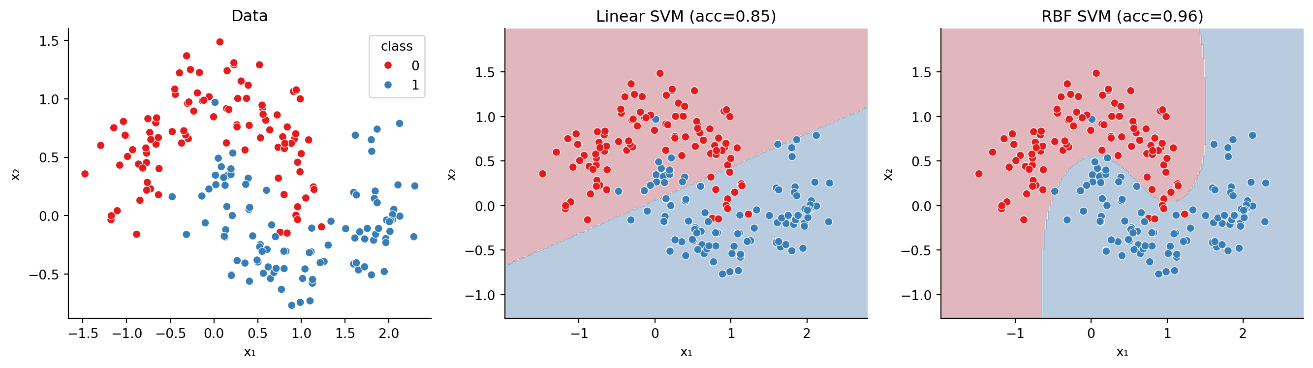
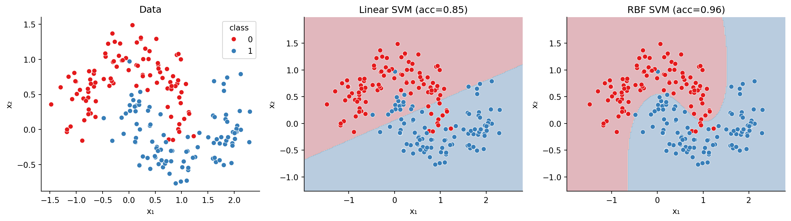
SVMs find the maximum-margin hyperplane separating classes — the decision boundary with the widest gap between the nearest points of each class (the “support vectors”). The kernel trick lets SVMs handle non-linear boundaries by implicitly mapping data to a higher-dimensional space:

\[ \hat{y} = \text{sign}\!\left(\sum_{i \in SV} \alpha_i \, y_i \, K(x_i, x) + b\right) \]

where \(K(x_i, x)\) is a kernel function (e.g. linear: \(x_i^\top x\), or RBF: \(\exp(-\gamma \|x_i - x\|^2)\)) and the sum is only over support vectors.

Code

# Generate non-linearly separable data
X_moons, y_moons = make_moons(n_samples=200, noise=0.2, random_state=42)

_moons_df = pl.DataFrame({
    "x1": X_moons[:, 0], "x2": X_moons[:, 1],
    "class": [str(c) for c in y_moons],
})

# Decision boundaries require contourf (matplotlib), so we use plt.subplots
# with sns.scatterplot layered on top
_fig, _axes = plt.subplots(1, 3, figsize=(14, 4))

for _ax, (_label, _kern) in zip(_axes, [("Data", None), ("Linear SVM", "linear"), ("RBF SVM", "rbf")]):
    if _kern is None:
        sns.scatterplot(data=_moons_df.to_pandas(), x="x1", y="x2", hue="class", palette="Set1", ax=_ax)
        _ax.set(title=_label)
    else:
        _svm = SVC(kernel=_kern).fit(X_moons, y_moons)
        _xx, _yy = np.meshgrid(
            np.linspace(X_moons[:, 0].min() - 0.5, X_moons[:, 0].max() + 0.5, 200),
            np.linspace(X_moons[:, 1].min() - 0.5, X_moons[:, 1].max() + 0.5, 200),
        )
        _ax.contourf(_xx, _yy, _svm.predict(np.c_[_xx.ravel(), _yy.ravel()]).reshape(_xx.shape), alpha=0.3, cmap="RdBu")
        sns.scatterplot(data=_moons_df.to_pandas(), x="x1", y="x2", hue="class", palette="Set1", ax=_ax, legend=False)
        _ax.set(title=f"{_label} (acc={_svm.score(X_moons, y_moons):.2f})")
    _ax.set(xlabel="x₁", ylabel="x₂")

plt.tight_layout()
sns.despine()
_fig

Code

# Pipeline: scale → classify → cross-validate
pipe_svm = make_pipeline(StandardScaler(), SVC(kernel="rbf"))
scores_svm = cross_val_score(pipe_svm, X_moons, y_moons, cv=5, scoring="accuracy")
print(f"SVM pipeline 5-fold accuracy: {scores_svm.mean():.3f} ± {scores_svm.std():.3f}")

SVM pipeline 5-fold accuracy: 0.955 ± 0.029

Naive Bayes

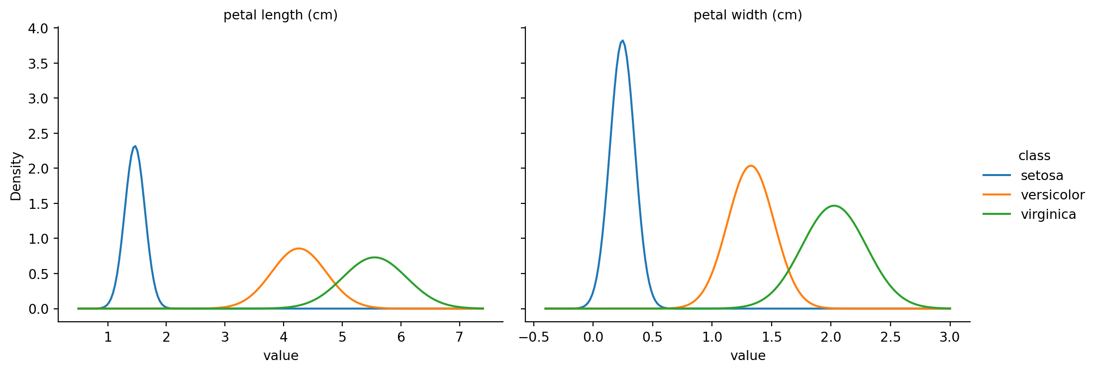
Naive Bayes uses Bayes’ theorem with a strong (“naive”) assumption: all features are conditionally independent given the class. Despite this simplification, it works surprisingly well for many problems, especially text classification:

\[ P(y \mid x_1, \ldots, x_p) \propto P(y) \prod_{j=1}^{p} P(x_j \mid y) \]

For continuous features, GaussianNB assumes each \(P(x_j \mid y)\) is a normal distribution with class-specific mean and variance.

Code

X_iris, y_iris = load_iris(return_X_y=True)
_iris_info = load_iris()

nb = GaussianNB()
nb.fit(X_iris, y_iris)

# Build long-format DataFrame of class-conditional Gaussian densities
_rows = []
for _feat_idx in [2, 3]:
    _feat_name = _iris_info.feature_names[_feat_idx]
    _x_range = np.linspace(X_iris[:, _feat_idx].min() - 0.5, X_iris[:, _feat_idx].max() + 0.5, 200)
    for _cls in range(3):
        _mu = nb.theta_[_cls, _feat_idx]
        _sigma = np.sqrt(nb.var_[_cls, _feat_idx])
        _density = (1 / (_sigma * np.sqrt(2 * np.pi))) * np.exp(-0.5 * ((_x_range - _mu) / _sigma) ** 2)
        for _x, _d in zip(_x_range, _density):
            _rows.append({"feature": _feat_name, "value": _x, "density": _d, "class": _iris_info.target_names[_cls]})

_nb_df = pl.DataFrame(_rows)

sns.relplot(
    data=_nb_df.to_pandas(),
    x="value", y="density",
    hue="class", col="feature",
    kind="line", height=4, aspect=1.3,
    facet_kws={"sharex": False},
).set_titles("{col_name}").set(ylabel="Density")

GaussianNB()

GaussianNB

?Documentation for GaussianNBiFitted

Parameters

	priors priors: array-like of shape (n_classes,), default=None Prior probabilities of the classes. If specified, the priors are not adjusted according to the data.	None
	var_smoothing var_smoothing: float, default=1e-9 Portion of the largest variance of all features that is added to variances for calculation stability. .. versionadded:: 0.20	1e-09

Fitted attributes

Name	Type	Value
class_count_ class_count_: ndarray of shape (n_classes,) number of training samples observed in each class.	ndarray[float64](3,)	[50.,50.,50.]
class_prior_ class_prior_: ndarray of shape (n_classes,) probability of each class.	ndarray[float64](3,)	[0.33,0.33,0.33]
classes_ classes_: ndarray of shape (n_classes,) class labels known to the classifier.	ndarray[int64](3,)	[0,1,2]
epsilon_ epsilon_: float absolute additive value to variances.	float64	3.096e-09
n_features_in_ n_features_in_: int Number of features seen during :term:`fit`. .. versionadded:: 0.24	int	4
theta_ theta_: ndarray of shape (n_classes, n_features) mean of each feature per class.	ndarray[float64](3, 4)	[[5.01,3.43,1.46,0.25], [5.94,2.77,4.26,1.33], [6.59,2.97,5.55,2.03]]
var_ var_: ndarray of shape (n_classes, n_features) Variance of each feature per class. .. versionadded:: 1.0	ndarray[float64](3, 4)	[[0.12,0.14,0.03,0.01], [0.26,0.1 ,0.22,0.04], [0.4 ,0.1 ,0.3 ,0.07]]

Code

# Pipeline: scale → classify → cross-validate
pipe_nb = make_pipeline(StandardScaler(), GaussianNB())
scores_nb = cross_val_score(pipe_nb, X_iris, y_iris, cv=5, scoring="accuracy")
print(f"NB pipeline 5-fold accuracy: {scores_nb.mean():.3f} ± {scores_nb.std():.3f}")

NB pipeline 5-fold accuracy: 0.953 ± 0.027

Cross-validation

Using bossanova

More generally using sklearn

Decomposition

Principal Components Analysis (PCA)

Factor Analysis

Independent Components Analysis (ICA)

Regularization

Ridge Regression

LASSO Regression

Classification

Support Vector Machines (SVM)

Naive Bayes

Using `bossanova`

More generally using `sklearn`