Mixed Models — Extending the GLM

Author

Eshin Jolly

Published

March 10, 2026

Code

# Import what we need
import polars as pl
from polars import col
import seaborn as sns
import numpy as np
from bossanova import model, compare, load_dataset

Over the past few notebooks we’ve built a solid GLM toolkit:

Parameter inference using asymptotic (formula), bootstrap, and permutation approaches with .infer(how='asym|boot|perm')
The marginal effects with the mixing board using .explore()
Generalized Linear Models like Logistic regression for binary outcomes using family='binomial'

Thus far, every model we’ve fit so far has assumed that each observation is independent — knowing one data point tells you nothing about another and therefore errors are independent & identitically distributed (iid) .

But that assumption breaks down all the time in real data:

The same person measured on multiple days (repeated measures)
trials nested within participants in an experiment
students nested within classrooms

When observations share a cluster they tend to be more similar to each other than to observations from other clusters. Ignoring this leads to overconfident estimates — your standard errors are too small and your p-values too optimistic.

The fix? Mixed models: they’re just another extension of the GLM you already know. Same model() function, same .explore() mixing board, same compare() for model comparison. We just add a new ingredient to the formula.

Simpson’s Paradox: Why Independence Matters

Before we get to the mechanics, let’s see why ignoring data structure can go badly wrong.

Here’s a simple dataset with 10 observations. There’s a variable x1235 and an outcome y. There’s also a column group which reflects which group repeated observations came from.

First, let’s fit a simple regression ignoring group:

Code

simpson = pl.read_csv("data/simpson.csv")
simpson.head()

shape: (5, 8)

x1235	y1	y2	y3	y5	x4	y4	group
f64	f64	f64	f64	f64	f64	f64	str
10.0	8.04	9.14	7.46	9.82	8.0	6.58	"A"
8.0	6.95	8.14	6.77	5.56	8.0	5.76	"B"
13.0	7.58	8.74	12.74	9.51	8.0	7.71	"A"
9.0	8.81	8.77	7.11	5.45	8.0	8.84	"B"
11.0	8.33	9.26	7.81	9.72	8.0	8.47	"A"

We can do this visually first using seaborn

Code

(
    sns.lmplot(
        data=simpson,
        x='x1235',
        y='y5',
        truncate=False,
        ci=None,
    )
    .set(ylim=(0,12), xlim=(0,20), xlabel='X', ylabel='Y', title='Complete Pooling')
)

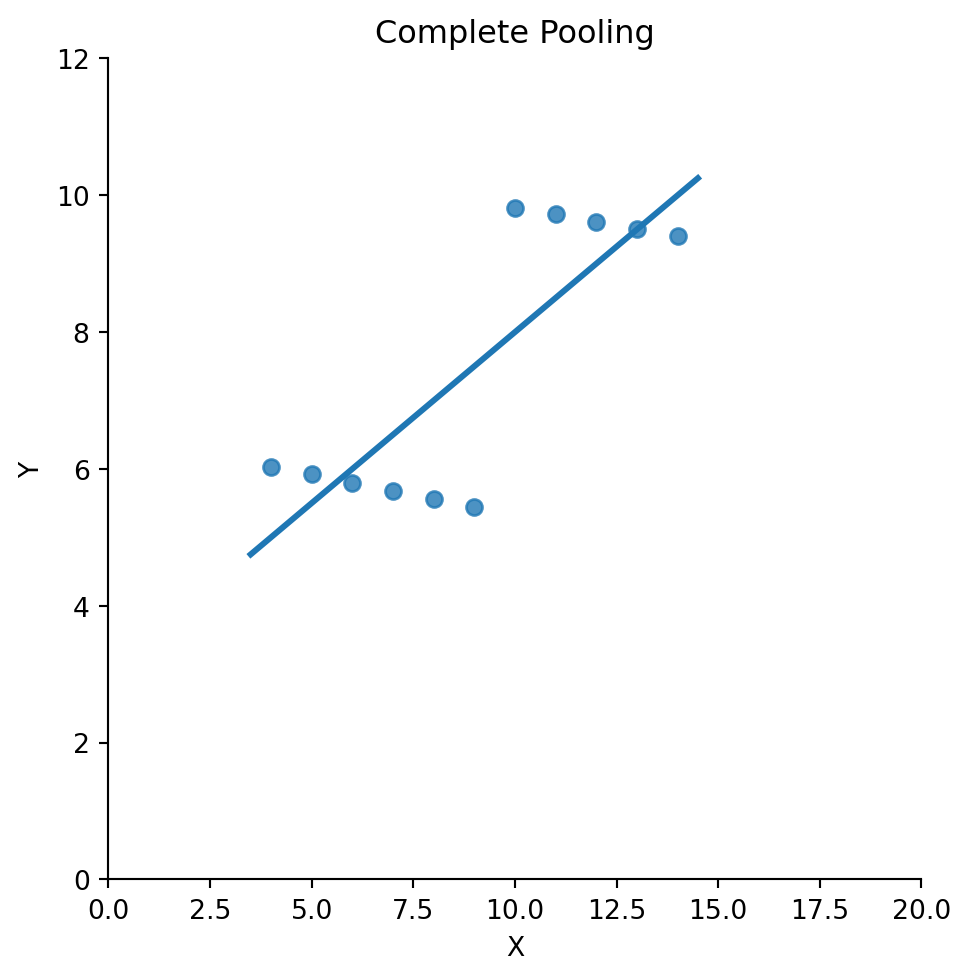
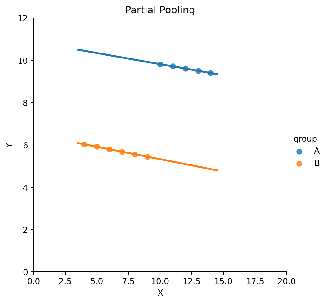
Notice how the regression slope is positive but the trend within each cluster is clearly negative

Lets estimate a model to confirm:

Tip: you can always chain the .summary() method to .fit(), .infer(), and .explore() to print an R style summary if you prefer that to polars dataframes accessible via .params and .effects

Code

model('y5 ~ x1235', data=simpson).fit().summary()

Linear Model: y5 ~ x1235

Residuals:
    Min      1Q  Median      3Q     Max
 -2.050  -0.710   0.011   0.820   1.820

Coefficients:
             Estimate
  Intercept     3.002
      x1235     0.500

Residual std error: 1.236 on 9 df
Multiple R-squared: 0.666, Adjusted R-squared: 0.629
AIC: 37.7, BIC: 38.5

Look at Coefficients: in the output above. Notice how the estimate for x1235 is positive?

Now we if we stratify data by the group column and re-plot/model we can see this trend reverse:

Code

(
    sns.lmplot(
        data=simpson,
        x='x1235',
        y='y5',
        hue='group',
        truncate=False,
    )
    .set(ylim=(0,12), xlim=(0,20), xlabel='X', ylabel='Y', title='Partial Pooling')
)

Code

# Fit a model with intercept per group
m2 = model('y5 ~ x1235 + (1 | group)', data=simpson).fit()

m2.summary()

Linear Mixed Model fit by REML: y5 ~ x1235 + (1 | group)
Number of obs: 11, groups:  group, 2

REML criterion at convergence: -36.436

Scaled residuals:
    Min      1Q  Median      3Q     Max
 -1.540  -0.570  -0.176   0.835   1.188

Varying effects:
 Groups    Name       Variance  Std.Dev.    Corr
 group     Intercept    10.040     3.169        
 Residual                0.000     0.011        
 ICC: 1.000

Fixed effects:
             Estimate
  Intercept     8.719
      x1235    -0.113

AIC: -30.4, BIC: -29.2

Look at the Fixed effects towards to bottom (same as .params):

By x1235 now has a negative estimate — the opposite of what the pooled regression told us!

This is Simpson’s Paradox: the overall trend reverses when you account for groups.

The problem is that participants differ in their baseline levels of both x and y. When we pool everyone together, those between-person differences create a spurious positive trend. This is exactly what happens when you violate the independence assumption — you confuse between-cluster variation with within-cluster effects.

Three Approaches to Clustered Data

Let’s work through a classic dataset to see how different approaches handle clustering. The sleep deprivation study (Belenky et al., 2003) measured reaction times for 18 participants over 10 days of sleep deprivation:

Variable	Description
Subject	Participant ID
Days	Days of sleep deprivation (0–9)
Reaction	Average reaction time (ms)

The question: How does sleep deprivation affect reaction time?

Code

sleep = load_dataset("sleep")
sleep.head()

shape: (5, 3)

Subject	Days	Reaction
i64	i64	f64
308	0	249.56
308	1	258.7047
308	2	250.8006
308	3	321.4398
308	4	356.8519

Code

sns.relplot(
    data=sleep.to_pandas(),
    x="Days",
    y="Reaction",
    hue="Subject",
    kind="line",
    height=4,
    aspect=1.5,
    palette="tab20",
    legend=False,
)

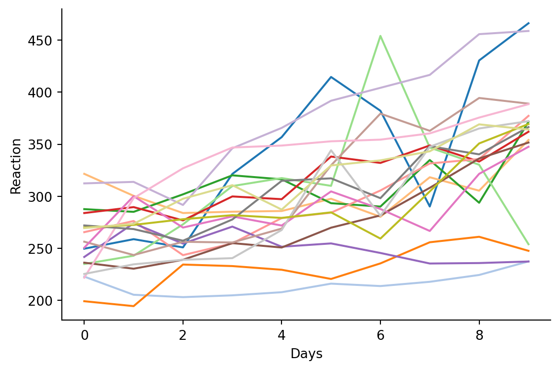
Notice two things:

Overall trend: reaction time increases with days of deprivation
Individual differences: some people start fast and stay fast, others start slow and get much slower

Let’s review the three approaches for dealing with dependent data we discussed in lecture:

Approach 1: Complete Pooling

Ignore the grouping entirely — fit one regression line through all 180 observations:

\[ Reaction_i = \beta_0 + \beta_1 \cdot Days_i + \epsilon_i \]

This is what we’ve been doing in every model so far. It assumes all observations are independent.

Code

m_complete = model("Reaction ~ Days", sleep).fit()
m_complete.params

shape: (2, 2)

term	estimate
str	f64
"Intercept"	251.4
"Days"	10.47

The model says reaction time increases by ~10.5 ms per day. But this estimate pretends all 180 data points are independent — it doesn’t know that groups of 10 come from the same person. The standard errors will be too small.

Approach 2: No Pooling

Fit a separate regression for each participant — 18 independent models:

Code

# Fit a separate model per subject
no_pool_results = []

# Loop over unique subjects
for subj in sleep.select("Subject").unique().sort("Subject").to_series():

    # Get just their data points
    subj_data = sleep.filter(pl.col("Subject") == subj)

    # Fit a model
    m = model("Reaction ~ Days", subj_data).fit()

    # Save estimates
    no_pool_results.append({
        "Subject": subj,
        "Intercept": m.params["estimate"][0],
        "Slope": m.params["estimate"][1],
    })

no_pool = pl.DataFrame(no_pool_results)
no_pool

shape: (18, 3)

Subject	Intercept	Slope
i64	f64	f64
308	244.2	21.76
309	205.1	2.262
310	203.5	6.115
330	289.7	3.008
331	285.7	5.266
…	…	…
352	276.4	13.57
369	255.0	11.35
370	210.4	18.06
371	253.6	9.188
372	267.0	11.3

Now each person gets their own intercept and slope. But this approach has problems too:

Subjects with noisy data get extreme estimates (no borrowing of information across people)
We can’t make population-level statements — we just have 18 separate stories
If someone has very few observations, their estimates are unreliable

Approach 3: Partial Pooling (Mixed Models)

The sweet spot. A mixed model estimates one population-level trend while allowing each participant to deviate from it:

\[ Reaction_{ij} = (\beta_0 + u_{0j}) + (\beta_1 + u_{1j}) \cdot Days_{ij} + \epsilon_{ij} \]

\(\beta_0, \beta_1\) are the fixed effects — the population average intercept and slope
\(u_{0j}, u_{1j}\) are the varying effects — how much subject \(j\) deviates from the population
The varying effects are assumed to come from a normal distribution: \(u_j \sim N(0, \tau^2)\)

This is called partial pooling because each person’s estimate is pulled (“shrunk”) toward the population average. People with noisy data get pulled more; people with clear patterns keep their individuality.

Random Intercepts

In bossanova and lme4 in R, varying effects term use the followin formula syntax:

Formula part	Meaning
`(1 \\| Subject)`	Random intercept only per `Subject`
`(0 + Days \\| Subject)`	Random slope only per `Subject`
`(1 \\| Subject) + (0 + Days \\| Subject)`	Random intercept + slope per `Subject`
`(Days \\| Subject)`	Random intercept + slope + correlation per `Subject`

Let’s start with random intercepts — each person can have a different baseline reaction time, but the effect of sleep deprivation is the same for everyone:

Code

m_ri = model("Reaction ~ Days + (1 | Subject)", sleep)
m_ri.fit()
m_ri.summary()

shape: (2, 2)

term	estimate
str	f64
"Intercept"	251.4
"Days"	10.47

Linear Mixed Model fit by REML: Reaction ~ Days + (1 | Subject)
Number of obs: 180, groups:  Subject, 18

REML criterion at convergence: 1786.465

Scaled residuals:
    Min      1Q  Median      3Q     Max
 -3.226  -0.553   0.011   0.519   4.251

Varying effects:
 Groups    Name       Variance  Std.Dev.    Corr
 Subject   Intercept  1378.179    37.124        
 Residual              960.457    30.991        
 ICC: 0.589

Fixed effects:
             Estimate
  Intercept   251.405
       Days    10.467

AIC: 1792.5, BIC: 1802.0

Let’s unpack the new parts of the output:

Fixed effects (.params) — same as before. The population-average intercept and slope:

Code

m_ri.params

shape: (2, 2)

term	estimate
str	f64
"Intercept"	251.4
"Days"	10.47

Variance components (.varying_spread) — how much variability is there between subjects?

Code

m_ri.varying_spread

shape: (5, 3)

term	metric	estimate
str	str	f64
"Subject \| Intercept"	"variance"	1378.0
"Subject \| Intercept"	"std_dev"	37.12
"ICC"	"icc"	0.5893
"Residual"	"variance"	960.5
"Residual"	"std_dev"	30.99

Subject | Intercept - variability around Subjects’ mean Reaction Time
ICC — intraclass correlation: the proportion of total variance that’s between subjects. Here ~0.59, meaning almost 60% of the variability in reaction time is due to who the person is, not how many days they’ve been deprived. That’s a lot of clustering!
Residual - error variance not accounted for by terms in the model

Subject-specific estimates (.varying_params) — also called the “best linear unbiased predictors” (BLUPs)

These are each subject’s intercept, after shrinkage toward the population mean. Notice how only the Intercept is different across participants beause we didn’t estimate a random slope. This is similar to the fixef(model) function in R:

Code

m_ri.varying_params

shape: (18, 3)

group	level	Intercept
str	str	f64
"Subject"	"308"	292.2
"Subject"	"309"	173.6
"Subject"	"310"	188.3
"Subject"	"330"	255.8
"Subject"	"331"	261.6
…	…	…
"Subject"	"352"	287.8
"Subject"	"369"	258.4
"Subject"	"370"	245.0
"Subject"	"371"	248.1
"Subject"	"372"	269.5

The .varying_offsets shows how much each person deviates from the population average (the varying effect itself). This the same as the ranef(model) function in R:

Code

m_ri.varying_offsets

shape: (18, 3)

group	level	Intercept
str	str	f64
"Subject"	"308"	40.78
"Subject"	"309"	-77.85
"Subject"	"310"	-63.11
"Subject"	"330"	4.406
"Subject"	"331"	10.22
…	…	…
"Subject"	"352"	36.38
"Subject"	"369"	7.036
"Subject"	"370"	-6.363
"Subject"	"371"	-3.294
"Subject"	"372"	18.12

Your Turn

Try estimating a model with intercepts, slopes, and their correlation using the formula refrence above. What do you see now in the model’s .varying_params?

Code

# Your code here

Code

# Your code here

How to Choose Varying Effects: Keep it Maximal

We’ve seen how to fit mixed models — but how do you decide which varying effects to include? The recommended approach (Barr et al., 2013) is:

Start maximal, then simplify.

Begin with the most complex random effects structure your design can support. If it doesn’t converge (or produces warnings), simplify step by step — using convergence diagnostics and model comparison to guide you.

Let’s walk through this process with a new dataset.

The cake dataset records the breakage angle of 3 cake recipes (A, B, C), each baked at 6 temperatures (175°–225°), with 15 replicates:

Code

cake = load_dataset("cake")
(
    sns.catplot(
        data=cake.to_pandas(),
        y='angle',
        x='recipe',
        hue='temperature',
        kind='box'
    )
)

1. Start with the maximal structure

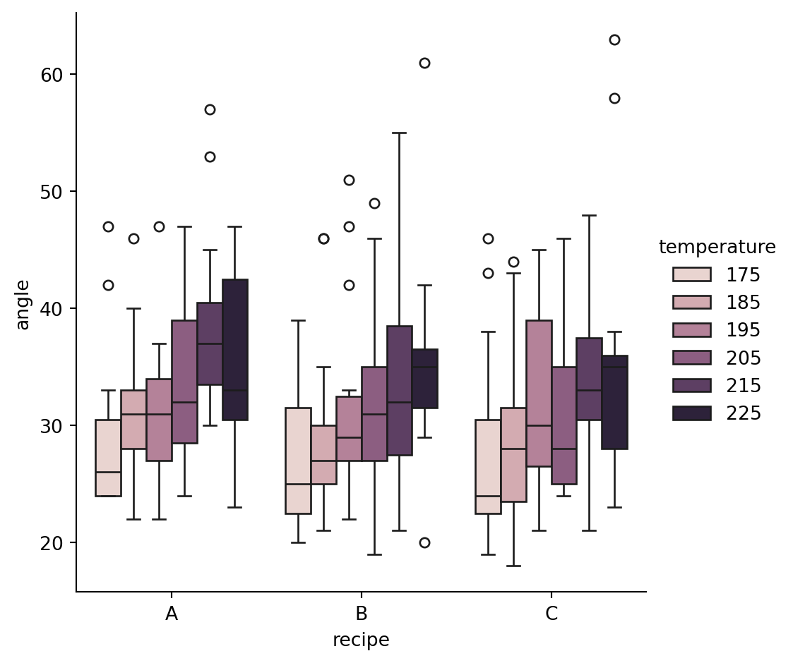
Each replicate saw all 3 recipes at all 6 temperatures — so both recipe and temperature are within-replicate factors. The maximal model lets each replicate have its own intercept, recipe effects, temperature slope, and recipe × temperature interactions:

Code

m_cake_max = model("angle ~ recipe * temperature + (recipe * temperature | replicate)", cake).fit()

2. Diagnose why convergence fails

The model fit, but those warnings tell us something important. Singular fit means some variance components were estimated at (essentially) zero — the model is trying to estimate more random variation than the data can support.

Let’s look at the variance components to see which ones collapsed:

Code

m_cake_max.varying_spread

shape: (30, 3)

term	metric	estimate
str	str	f64
"replicate \| Intercept"	"variance"	194.9
"replicate \| Intercept"	"std_dev"	13.96
"replicate \| recipe[B]"	"variance"	341.6
"replicate \| recipe[B]"	"std_dev"	18.48
"replicate \| recipe[C]"	"variance"	252.2
…	…	…
"temperature:recipe[C]:temperat…	"corr"	-0.7386
"recipe[B]:temperature:recipe[C…	"corr"	0.5957
"ICC"	"icc"	0.6923
"Residual"	"variance"	19.37
"Residual"	"std_dev"	4.401

3. Simplify starting with higher-order terms

The interaction slopes have near-zero variance — replicates don’t differ in their recipe × temperature interactions. Follow the hierarchy: drop interactions first, then slopes, then correlations:

Code

# Drop interaction from RE
m_cake_add = model("angle ~ recipe * temperature + (recipe + temperature | replicate)", cake).fit()

Code

m_cake_add.varying_spread

shape: (17, 3)

term	metric	estimate
str	str	f64
"replicate \| Intercept"	"variance"	40.72
"replicate \| Intercept"	"std_dev"	6.381
"replicate \| recipe[B]"	"variance"	7.504
"replicate \| recipe[B]"	"std_dev"	2.739
"replicate \| recipe[C]"	"variance"	14.59
…	…	…
"recipe[B]:temperature"	"corr"	0.2054
"recipe[C]:temperature"	"corr"	-0.07784
"ICC"	"icc"	0.6793
"Residual"	"variance"	20.14
"Residual"	"std_dev"	4.488

Code

# Drop temperature slope (near-zero in additive model too)
m_cake_recipe = model("angle ~ recipe * temperature + (recipe | replicate)", cake).fit()

Code

m_cake_recipe.varying_spread

shape: (12, 3)

term	metric	estimate
str	str	f64
"replicate \| Intercept"	"variance"	26.89
"replicate \| Intercept"	"std_dev"	5.185
"replicate \| recipe[B]"	"variance"	7.103
"replicate \| recipe[B]"	"std_dev"	2.665
"replicate \| recipe[C]"	"variance"	14.33
…	…	…
"Intercept:recipe[C]"	"corr"	0.2989
"recipe[B]:recipe[C]"	"corr"	0.9905
"ICC"	"icc"	0.6684
"Residual"	"variance"	20.78
"Residual"	"std_dev"	4.558

Code

# Drop correlation between slope and interept for recipe
m_cake_recipe_nocorr = model("angle ~ recipe * temperature + (1 | replicate) + (0 + recipe | replicate)", cake).fit()

Code

m_cake_recipe_nocorr.varying_spread

shape: (9, 3)

term	metric	estimate
str	str	f64
"replicate \| Intercept"	"variance"	33.45
"replicate \| Intercept"	"std_dev"	5.783
"replicate \| recipe[B]"	"variance"	3.397
"replicate \| recipe[B]"	"std_dev"	1.843
"replicate \| recipe[C]"	"variance"	8.684
"replicate \| recipe[C]"	"std_dev"	2.947
"ICC"	"icc"	0.6385
"Residual"	"variance"	21.21
"Residual"	"std_dev"	4.606

Just for comparison purposes lets also estimate a random-intercepts only model

Code

# Random intercepts only
m_cake_ri = model("angle ~ recipe * temperature + (1 | replicate)", cake).fit()

Code

m_cake_ri.varying_spread

shape: (5, 3)

term	metric	estimate
str	str	f64
"replicate \| Intercept"	"variance"	39.2
"replicate \| Intercept"	"std_dev"	6.261
"ICC"	"icc"	0.6268
"Residual"	"variance"	23.34
"Residual"	"std_dev"	4.831

4. Use model comparison (`compare()`)

Now we use compare() to test whether the added complexity is “worth it.” For mixed models, compare() uses a likelihood ratio test instead of an F-test.

You can see that our maximal model has 28 parameters while our simplest model has only 8. The p-value column compares successive models and is suggsting we might still consider there’s an improvement from the m_cake_ri (intercept only) model which successfully converged and the m_cake_recipe_nocorr model:

Code

compare(m_cake_ri,m_cake_recipe_nocorr, m_cake_recipe, m_cake_add, m_cake_max)

shape: (5, 9)

model	chi2	npar	AIC	BIC	loglik	deviance	df	p_value
str	f64	i64	f64	f64	f64	f64	i64	f64
"angle ~ recipe * temperature +…	null	8	1689.0	1718.0	-836.5	1673.0	null	null
"angle ~ recipe * temperature +…	6.124	10	1687.0	1723.0	-833.5	1667.0	2	0.0468
"angle ~ recipe * temperature +…	10.66	13	1682.0	1729.0	-828.1	1656.0	3	0.01371
"angle ~ recipe * temperature +…	2.961	17	1687.0	1748.0	-826.7	1653.0	4	0.5643
"angle ~ recipe * temperature +…	2.291	28	1707.0	1808.0	-825.5	1651.0	11	0.9972

Let’s look at the diagnostics for those 2 models specifically:

Code

# Intercept only
m_cake_ri.diagnostics

shape: (1, 11)

df_model	df_resid	sigma	deviance	mse	rsquared_marginal	rsquared_conditional	icc	aic	bic	loglik
f64	f64	f64	f64	f64	f64	f64	f64	f64	f64	f64
5.0	264.0	4.831	1673.0	21.65	0.1108	0.6681	0.6268	1689.0	1718.0	-836.5

Code

# Recipe intercept, slope, but no correlation
m_cake_recipe_nocorr.diagnostics

shape: (1, 11)

df_model	df_resid	sigma	deviance	mse	rsquared_marginal	rsquared_conditional	icc	aic	bic	loglik
f64	f64	f64	f64	f64	f64	f64	f64	f64	f64	f64
5.0	264.0	4.606	1667.0	18.65	0.1045	0.7154	0.6821	1687.0	1723.0	-833.5

The mse for the second model is a bit lower and adding the 2 additional parameters improves the fit.

5. Now use `jointtest()` and `explore()` to understand fixed effects

With the varying effects structure settled, return to the same workflow as before — the formula changes, the analysis doesn’t:

Since we’re just exploring this dataset and don’t have strong hypothesis lets run omnibus F-tests:

Code

m_cake_recipe_nocorr.jointtest()

shape: (3, 5)

term	df1	df2	f_ratio	p_value
str	i64	f64	f64	f64
"recipe"	2	264.0	0.102038	0.903031
"temperature"	1	264.0	92.705488	2.2204e-16
"recipe:temperature"	2	264.0	0.041047	0.95979

You just ran a “repeated measures ANOVA”! And it shows a clear main effect of temperature!

Now let’s use .explore() just like we’ve done to see how model predictions change for different temperature levels:

Code

m_cake_recipe_nocorr.explore("temperature@[175, 185, 195, 205, 215, 225]").infer().effects

shape: (6, 8)

temperature	estimate	se	ci_lower	ci_upper	statistic	df	p_value
i64	f64	f64	f64	f64	f64	f64	f64
175	28.17	1.602	24.78	31.56	17.59	16.28	5.1480e-12
185	29.75	1.568	26.41	33.09	18.97	14.96	7.0950e-12
195	31.33	1.551	28.01	34.65	20.21	14.32	6.3030e-12
205	32.91	1.551	29.59	36.23	21.22	14.32	3.1830e-12
215	34.49	1.568	31.15	37.84	22.0	14.96	8.3530e-13
225	36.07	1.602	32.68	39.46	22.52	16.28	1.0710e-13

Summary

Starting maximal and simplifying is a process, not a recipe. The convergence warnings told us the data couldn’t support all those random slopes — and compare() confirmed that the simpler structure fit just as well. In practice, this means the differences between replicates are mostly about baseline breakage angle, not about how recipes or temperatures affect breakage differently across replicates. The RM-ANOVA connection: A mixed model with a categorical fixed effect and random intercepts per subject is equivalent to a repeated-measures ANOVA. The .jointtest() F-test and the RM-ANOVA F-test will give you the same answer. But mixed models are more flexible — they handle unbalanced designs, missing data, continuous predictors, and complex varying effects structures that RM-ANOVA cannot.

Mixed models extend the GLM to handle clustered data — repeated measures, nested observations, or any situation where independence is violated.

What you already knew	What’s new
`model("y ~ x", data)`	`model("y ~ x + (1 \\| group)", data)`
`.params` — fixed effects	`.varying_params` — group-specific estimates
`.explore()` — marginal predictions	Same! (population-averaged)
`.jointtest()` — omnibus F-test	Same! (≈ repeated-measures ANOVA)
`compare(m1, m2)` — F-test	`compare(m1, m2)` — likelihood ratio test
`family="binomial"` — logistic	`family="binomial" + (1 \\| group)` — GLMM

The core insight: the formula changes, the workflow doesn’t.

Your Turn: Growth Curves

The chickweight dataset tracks the weight of 50 chicks over 12 timepoints (days 0–21), with each chick assigned to one of 4 diets:

chick = load_dataset("chickweight")

Follow the same 5-step workflow:

Start maximal: weight ~ Time * Diet + (Time * Diet | Chick) — what happens?
Diagnose: Why does it fail? (Hint: is Diet a within-Chick or between-Chick variable?)
Simplify: What’s the most complex structure that makes sense given the design?
Compare: Use compare() to pick the best varying effects structure
Infer: Use jointtest() and explore() on your best model

Feel free to make any visualizations to help you out!

Code

# Step 1: Load data and try maximal model

Code

# Step 2: Diagnose

Code

# Step 3: Simplify

Code

# Step 4: Compare

Code

# Step 5: Fixed effects inference

Your interpretation here: What did you learn about the diet effects on chick growth? Why couldn’t the maximal model work?

Simpson’s Paradox: Why Independence Matters

Three Approaches to Clustered Data

Approach 1: Complete Pooling

Approach 2: No Pooling

Approach 3: Partial Pooling (Mixed Models)

Random Intercepts

Your Turn

How to Choose Varying Effects: Keep it Maximal

1. Start with the maximal structure

2. Diagnose why convergence fails

3. Simplify starting with higher-order terms

4. Use model comparison (compare())

5. Now use jointtest() and explore() to understand fixed effects

Summary

Your Turn: Growth Curves

4. Use model comparison (`compare()`)

5. Now use `jointtest()` and `explore()` to understand fixed effects