Introduction to numpy

Introduction to `numpy`#

Welcome to the absolute beginner’s guide to NumPy!

NumPy (Numerical Python) is an open source Python library that’s widely used in science and engineering. The NumPy library contains multidimensional array data structures, such as the homogeneous, N-dimensional ndarray, and a large library of functions that operate efficiently on these data structures.

How to use this notebook#

This notebook is designed for you to work through at your own pace. When you’re finished you should save and commit your changes and push them to your Github Classroom repository

Try experimenting by creating new code cells and playing around with the demonstrated functionality.

As you go through this notebook and work on the mini-exercises and challenge at the end, you might find the additional resources helpful:

How to import NumPy#

We can make numpy available by using the import statement. It’s convention to import numpy in the following way:

import numpy as np

A note on reading `numpy` documentation online#

As you go through this notebook, you should regularly refer to the numpy documentation to look things up and general help.

Throughout the documentation website, you will find blocks that look like:

>>> a = np.array([[1, 2, 3],
...               [4, 5, 6]])
>>> a.shape
(2, 3)

Text after any >>> or ... is input. This is the code you should copy or type into your notebook to try things out.

>>> and ... are not part of the code and will cause an error if entered into a notebook cell!

A note on accessing help from within this notebook#

When it comes to the data science ecosystem, Python and NumPy are built with the user in mind. One of the best examples of this is the built-in access to documentation. Every object contains the reference to a string, which is known as the docstring. In most cases, this docstring contains a quick and concise summary of the object and how to use it. Python has a built-in help() function that can help you access this information. This means that nearly any time you need more information, you can use help() to quickly find the information that you need.

For example:

help(max)

Help on built-in function max in module builtins:

max(...)
    max(iterable, *[, default=obj, key=func]) -> value
    max(arg1, arg2, *args, *[, key=func]) -> value
    
    With a single iterable argument, return its biggest item. The
    default keyword-only argument specifies an object to return if
    the provided iterable is empty.
    With two or more arguments, return the largest argument.

Because access to additional information is so useful, Interaactive Python uses the ? character as a shorthand for accessing this documentation along with other relevant information.

For example:

max?

Docstring:
max(iterable, *[, default=obj, key=func]) -> value
max(arg1, arg2, *args, *[, key=func]) -> value

With a single iterable argument, return its biggest item. The
default keyword-only argument specifies an object to return if
the provided iterable is empty.
With two or more arguments, return the largest argument.
Type:      builtin_function_or_method

You can even use this notation for object methods and objects themselves.

Let’s say you create this array:

a = np.array([1, 2, 3, 4, 5, 6])

Then you can obtain a lot of useful information (first details about a itself, followed by the docstring of ndarray of which a is an instance):

a?

Type:        ndarray
String form: [1 2 3 4 5 6]
Length:      6
File:        ~/miniconda3/envs/201b/lib/python3.11/site-packages/numpy/__init__.py
Docstring:  
ndarray(shape, dtype=float, buffer=None, offset=0,
        strides=None, order=None)

An array object represents a multidimensional, homogeneous array
of fixed-size items.  An associated data-type object describes the
format of each element in the array (its byte-order, how many bytes it
occupies in memory, whether it is an integer, a floating point number,
or something else, etc.)

Arrays should be constructed using `array`, `zeros` or `empty` (refer
to the See Also section below).  The parameters given here refer to
a low-level method (`ndarray(...)`) for instantiating an array.

For more information, refer to the `numpy` module and examine the
methods and attributes of an array.

Parameters
----------
(for the __new__ method; see Notes below)

shape : tuple of ints
    Shape of created array.
dtype : data-type, optional
    Any object that can be interpreted as a numpy data type.
buffer : object exposing buffer interface, optional
    Used to fill the array with data.
offset : int, optional
    Offset of array data in buffer.
strides : tuple of ints, optional
    Strides of data in memory.
order : {'C', 'F'}, optional
    Row-major (C-style) or column-major (Fortran-style) order.

Attributes
----------
T : ndarray
    Transpose of the array.
data : buffer
    The array's elements, in memory.
dtype : dtype object
    Describes the format of the elements in the array.
flags : dict
    Dictionary containing information related to memory use, e.g.,
    'C_CONTIGUOUS', 'OWNDATA', 'WRITEABLE', etc.
flat : numpy.flatiter object
    Flattened version of the array as an iterator.  The iterator
    allows assignments, e.g., ``x.flat = 3`` (See `ndarray.flat` for
    assignment examples; TODO).
imag : ndarray
    Imaginary part of the array.
real : ndarray
    Real part of the array.
size : int
    Number of elements in the array.
itemsize : int
    The memory use of each array element in bytes.
nbytes : int
    The total number of bytes required to store the array data,
    i.e., ``itemsize * size``.
ndim : int
    The array's number of dimensions.
shape : tuple of ints
    Shape of the array.
strides : tuple of ints
    The step-size required to move from one element to the next in
    memory. For example, a contiguous ``(3, 4)`` array of type
    ``int16`` in C-order has strides ``(8, 2)``.  This implies that
    to move from element to element in memory requires jumps of 2 bytes.
    To move from row-to-row, one needs to jump 8 bytes at a time
    (``2 * 4``).
ctypes : ctypes object
    Class containing properties of the array needed for interaction
    with ctypes.
base : ndarray
    If the array is a view into another array, that array is its `base`
    (unless that array is also a view).  The `base` array is where the
    array data is actually stored.

See Also
--------
array : Construct an array.
zeros : Create an array, each element of which is zero.
empty : Create an array, but leave its allocated memory unchanged (i.e.,
        it contains "garbage").
dtype : Create a data-type.
numpy.typing.NDArray : An ndarray alias :term:`generic <generic type>`
                       w.r.t. its `dtype.type <numpy.dtype.type>`.

Notes
-----
There are two modes of creating an array using ``__new__``:

1. If `buffer` is None, then only `shape`, `dtype`, and `order`
   are used.
2. If `buffer` is an object exposing the buffer interface, then
   all keywords are interpreted.

No ``__init__`` method is needed because the array is fully initialized
after the ``__new__`` method.

Examples
--------
These examples illustrate the low-level `ndarray` constructor.  Refer
to the `See Also` section above for easier ways of constructing an
ndarray.

First mode, `buffer` is None:

>>> np.ndarray(shape=(2,2), dtype=float, order='F')
array([[0.0e+000, 0.0e+000], # random
       [     nan, 2.5e-323]])

Second mode:

>>> np.ndarray((2,), buffer=np.array([1,2,3]),
...            offset=np.int_().itemsize,
...            dtype=int) # offset = 1*itemsize, i.e. skip first element
array([2, 3])

This also works for functions and other objects that you create. Just remember to include a docstring with your function using a string literal (""" """ or ''' ''' around your documentation).

For example, if you create this function:

def double(a):
    '''Return a * 2'''
    return a * 2

You can obtain information about the function:

double?

Signature: double(a)
Docstring: Return a * 2
File:      /var/folders/4y/y26_jdm57m90f4s1td24ls040000gn/T/ipykernel_54391/2713554790.py
Type:      function

Which prints out your docstring!

You can reach another level of information by reading the source code of the object you’re interested in. Using a double question mark (??) allows you to access the source code.

For example:

double??

Signature: double(a)
Source:   
def double(a):
    '''Return a * 2'''
    return a * 2
File:      /var/folders/4y/y26_jdm57m90f4s1td24ls040000gn/T/ipykernel_54391/2713554790.py
Type:      function

Which prints out your source code!

Why use NumPy?#

Python lists are excellent, general-purpose containers. They can be “heterogeneous”, meaning that they can contain elements of a variety of types, and they are quite fast when used to perform individual operations on a handful of elements.

Depending on the characteristics of the data and the types of operations that need to be performed, other containers may be more appropriate; by exploiting these characteristics, we can improve speed, reduce memory consumption, and offer a high-level syntax for performing a variety of common processing tasks. NumPy shines when there are large quantities of “homogeneous” (same-type) data to be processed on the CPU.

What is an “array”?#

In computer programming, an array is a structure for storing and retrieving data. We often talk about an array as if it were a grid in space, with each cell storing one element of the data. For instance, if each element of the data were a number, we might visualize a “one-dimensional” array like a list:

\[\begin{split}\begin{aligned} \begin{array}{|c||c|c|c|} \hline 1 & 5 & 2 & 0 \\ \hline \end{array} \end{aligned}\end{split}\]

A two-dimensional array would be like a table:

\[\begin{split}\begin{aligned} \begin{array}{|c||c|c|c|} \hline 1 & 5 & 2 & 0 \\ \hline 8 & 3 & 6 & 1 \\ \hline 1 & 7 & 2 & 9 \\ \hline \end{array} \end{aligned}\end{split}\]

A three-dimensional array would be like a set of tables, perhaps stacked as though they were printed on separate pages. In NumPy, this idea is generalized to an arbitrary number of dimensions, and so the fundamental array class is called ndarray: it represents an “N-dimensional array”.

Most NumPy arrays have some restrictions. For instance:

All elements of the array must be of the same type of data.
Once created, the total size of the array can’t change.
The shape must be “rectangular”, not “jagged”; e.g., each row of a two-dimensional array must have the same number of columns.

When these conditions are met, NumPy exploits these characteristics to make the array faster, more memory efficient, and more convenient to use than less restrictive data structures.

For the remainder of this notebook, we will use the word “array” to refer to an instance of ndarray.

Array fundamentals#

One way to initialize an array is using a Python sequence, such as a list. For example:

a = np.array([1, 2, 3, 4, 5, 6])
a

The code above is equivalent to creating to first creating a regular Python list, saving it to a variable, and then passing that variable to the np.array() function.

my_list = [1, 2, 3, 4, 5, 6]
a = np.array(my_list)
a

Elements of an array can be accessed in by indexing and slicing similar to normal lists or iterables in Python (e.g. strings).

For instance, we can access an individual element of this array as we would access an element in the original list: using the integer index of the element within square brackets.

a[0]

As with built-in Python sequences, NumPy arrays are “0-indexed”: the first element of the array is accessed using index 0, not 1.

Also like a Python list, arrays are mutable which means we can change their contents after they are created.

a[0] = 10
a

Also like the original list, Python slice notation can be used for indexing.

a[:3]

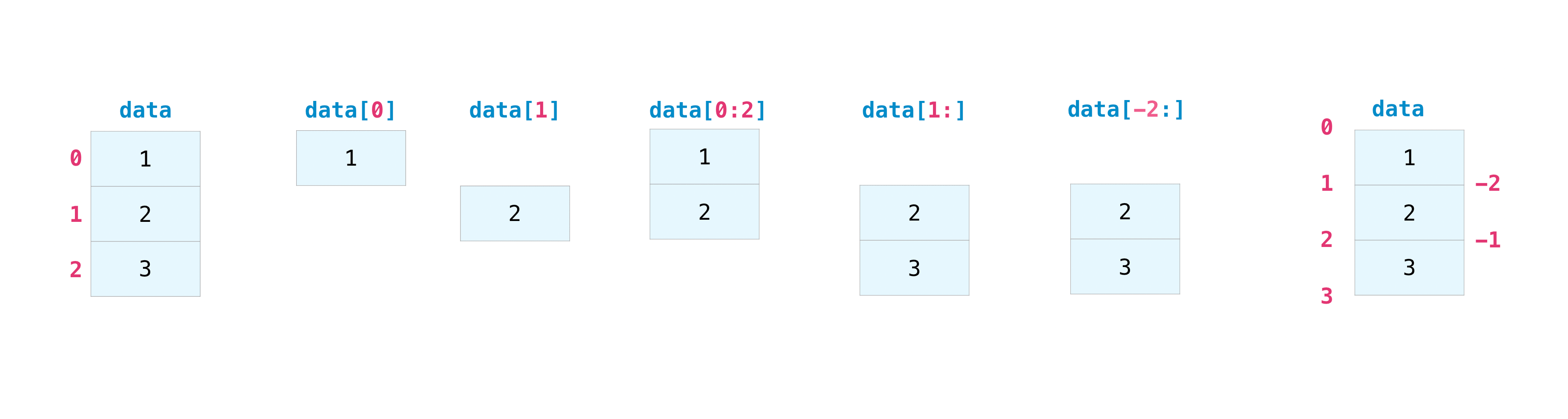
It may be helpful to visualize how the following slicing operations work:

>>> data = np.array([1, 2, 3])

>>> data[1]
2
>>> data[0:2]
array([1, 2])
>>> data[1:]
array([2, 3])
>>> data[-2:]
array([2, 3])

Arrays vs Lists: Views#

One major difference is that slice indexing of a list copies the elements into a new list, but slicing an array returns a view: an object that refers to the data in the original array.

That means the original array can be changed using the view.

b = a[3:]
b

b[0] = 40
a

Views are an important NumPy concept! NumPy functions, as well as operations like indexing and slicing, will return views whenever possible. This saves memory and is faster (no copy of the data has to be made). However it’s important to be aware of this - modifying data in a view also modifies the original array!

Using the copy method instead, will make a complete copy of the array and its data (a deep copy). To use this on your array, you could run:

b2 = a.copy()
b2

See the copies-and-views documentation for a more comprehensive explanation of when array operations return views rather than copies.

Boolean indexing#

If you want to select values from your array that fulfill certain True/Falseconditions, it’s straightforward with NumPy and we refer to this as boolean indexing.

For example, if you start with this array:

a = np.array([[1 , 2, 3, 4], [5, 6, 7, 8], [9, 10, 11, 12]])
a

You can easily print all of the values in the array that are less than 5. :

a[a < 5]

A common pattern in numpy is to create a variable that stores a Boolean mask that you can use to index the array like above. This is handy if you want to subset values in different arrays using the same condition. Let’s create a new array b and use a mask to index into both a and b in the same way:

b = a + 1
b

mask = a % 2 == 0 # even numbers
mask

# Even values in a
a[mask]

# Corresponding values in b where *a is even*
# *not* the even values in b!
b[mask]

You can select elements that satisfy two conditions using the & (and) and | (or) operators:

c = a[(a > 2) & (a < 11)]
c

And of course you can use these operators to create boolean mask arrays:

five_up = (a > 5) | (a == 5) # mask

five_up

b[five_up]

Two- and higher-dimensional arrays can be initialized from nested Python lists:

nested_list = [[1, 2, 3, 4], [5, 6, 7, 8], [9, 10, 11, 12]]
a = np.array(nested_list)
a

In NumPy, a dimension of an array is sometimes referred to as an “axis”. This terminology may be useful to disambiguate between the dimensionality of an array and the dimensionality of the data represented by the array. For instance, the array a could represent three points, each lying within a four-dimensional space, but a has only two “axes”.

Another difference between an array and a list of lists is that an element of the array can be accessed by specifying the index along each axis within a single set of square brackets, separated by commas. For instance, the element 8 is in row 1 and column 3:

a[1,3]

You can also use np.nonzero() to return a list of indices where elements are. This is another way to generate a “mask” array for re-use:

Starting with this array:

a = np.array([[1, 2, 3, 4], [5, 6, 7, 8], [9, 10, 11, 12]])
a

b = np.nonzero(a < 5)
b

a[b]

In this example, a tuple of arrays was returned: one for each dimension. The first array represents the row indices where these values are found, and the second array represents the column indices where the values are found.

If you want to generate a list of coordinates where the elements exist, you can zip the arrays, iterate over the list of coordinates, and print them. For example:

list_of_coordinates= list(zip(b[0], b[1]))
for coord in list_of_coordinates:
    print(coord)

If the element you’re looking for doesn’t exist in the array, then the returned array of indices will be empty. For example:

np.nonzero(a == 42)

A note on indexing#

It is familiar practice in mathematics to refer to elements of a matrix by the row index first and the column index second. This happens to be true for two-dimensional arrays.

But a better mental model is to think of the column index as the last and the row index as second to last. This generalizes to arrays with any number of dimensions.

# A 3-dimensional array
b = np.array(
    [
        [
            [1, 2, 3], 
            [4, 5, 6], 
            [7, 8, 9]
         ],
        [
            [10, 11, 12], 
            [13, 14, 15], 
            [16, 17, 18]
        ],
        [
            [19, 20, 21],
            [22, 23, 24],
            [25, 26, 27]],
    ]
)

row_idx = 1 # the 2nd row
col_idx = 2 # the 3rd column

# 0 is getting the first element in the 
# non-row, non-column dimension
# which "block" of 3x3 arrays, we're looking in
b[0, row_idx, col_idx]

A note on terminology#

You’ll often hear of a 0-D (zero-dimensional) array referred to as a “scalar”, a 1-D (one-dimensional) array as a “vector”, a 2-D (two-dimensional) array as a “*matrix”,an N-D (N-dimensional, where “N” is typically an integer greater than 2) array as a “tensor”.

For clarity, it is best to avoid the mathematical terms when referring to an array because the mathematical objects with these names behave differently than arrays (e.g. “matrix” multiplication is fundamentally different from “array” multiplication), and there are other objects in the scientific Python ecosystem that have these names (e.g. the fundamental data structure of PyTorch an immensely popular Deep-Learning library, is the “tensor”).

Array attributes#

This section covers the ndim, shape, size, and dtype attributes of an array.

ndarray.ndim will tell you the number of axes, or dimensions, of the array.

ndarray.size will tell you the total number of elements of the array. This is the product of the elements of the array’s shape.

ndarray.shape will display a tuple of integers that indicate the number of elements stored along each dimension of the array. If, for example, you have a 2-D array with 2 rows and 3 columns, the shape of your array is (2, 3).

The number of dimensions of an array is contained in the ndim attribute.

a.ndim

The shape of an array is a tuple of non-negative integers that specify the number of elements along each dimension.

a.shape

len(a.shape) == a.ndim

The fixed, total number of elements in array is contained in the size attribute.

a.size

import math

a.size == math.prod(a.shape)

Arrays are typically “homogeneous”, meaning that they contain elements of only one “data type”. The data type is recorded in the dtype attribute.

a.dtype # int for integer, "64" for 64-bit based on your OS

You can read more about array attributes here and learn about the array object here

Array operations#

Once you’ve created your arrays, you can start to work with them. Let’s say, for example, that you’ve created two arrays, one called “data” and one called “ones”

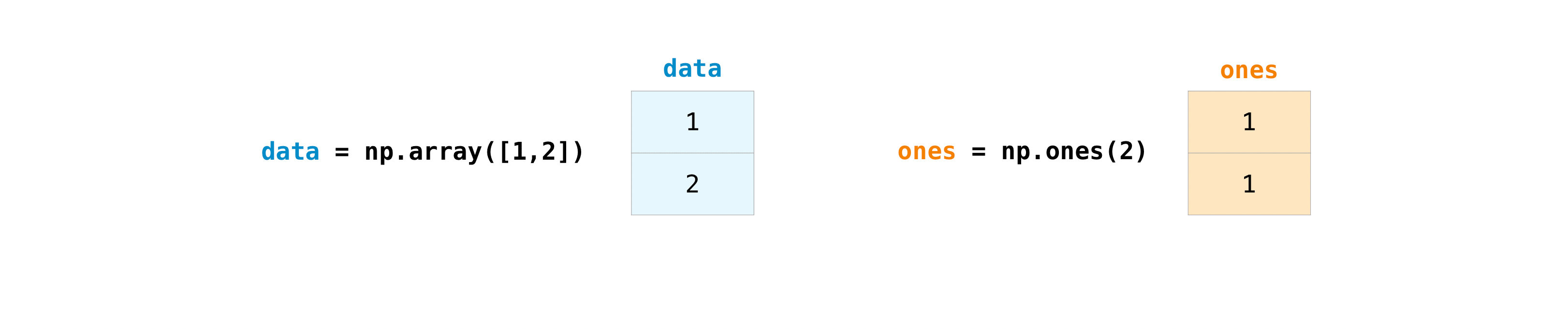
You can add the arrays together with the + operator

data = np.array([1, 2])
ones = np.ones(2, dtype=int)
data + ones

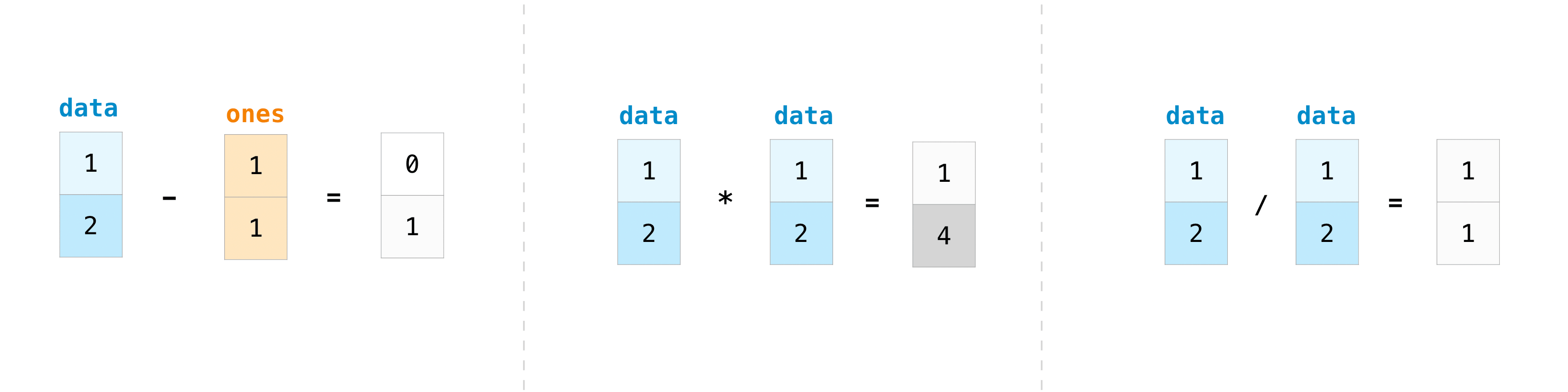
Of course you can do more than addition:

data - ones

data * data

data / data

Basic operations are simple with NumPy. If you want to find the sum of the elements in an array, you’d use sum(). This works for 1D arrays, 2D arrays, and arrays in higher dimensions. :

a = np.array([1, 2, 3, 4])
a.sum()

To add the rows or the columns in a 2D array, you would specify the axis.

If you start with this array:

b = np.array([[1, 1], [2, 2]])
b

You can sum over the axis of rows with:

b.sum(axis=0)

You can sum over the axis of columns with:

b.sum(axis=1)

Broadcasting#

There are times when you might want to carry out an operation between an array and a single number (also called an operation between a vector and a scalar) or between arrays of two different sizes. For example, your array (we’ll call it “data”) might contain information about distance in miles but you want to convert the information to kilometers. You can perform this operation with:

data = np.array([1.0, 2.0])
data * 1.6

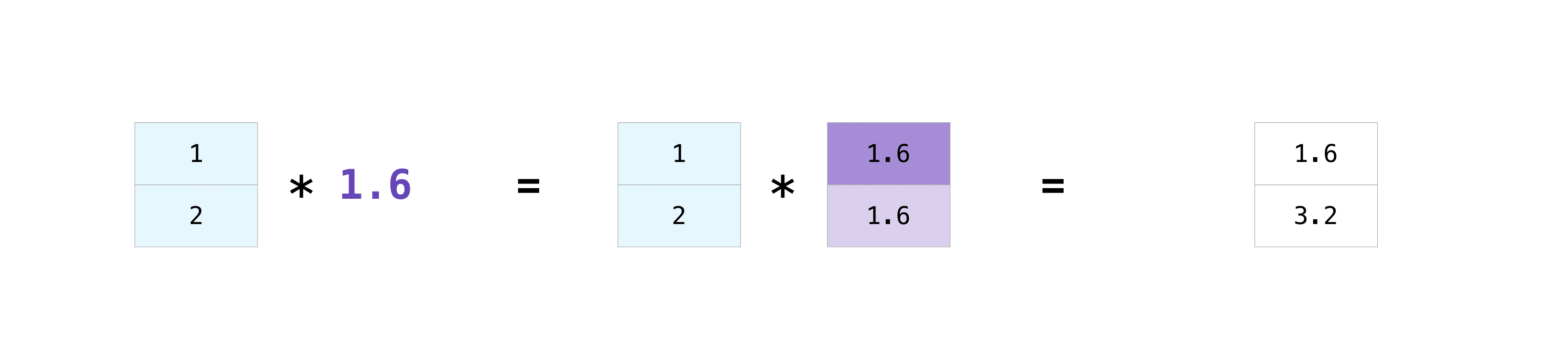
NumPy understands that the multiplication should happen with each cell. That concept is called broadcasting. Broadcasting is a mechanism that allows NumPy to perform operations on arrays of different shapes. The dimensions of your array must be compatible, for example, when the dimensions of both arrays are equal or when one of them is 1. If the dimensions are not compatible, you will get a ValueError.

Note on difference with lists#

You can now see how we can avoid using for loops to do operations because numpy arrays will perform vectorized operations for us. In other words, we can do operations on entire arrays at once.

More useful array operations#

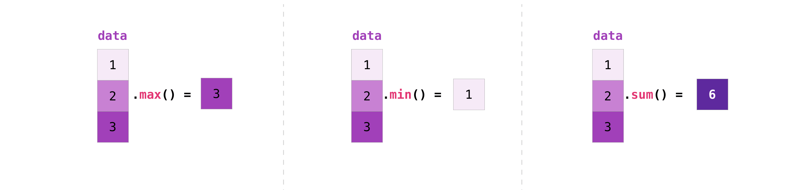
NumPy also performs aggregation functions. In addition to min, max, and sum, you can easily run mean to get the average, prod to get the result of multiplying the elements together, std to get the standard deviation, and more. :

data.max()

data.min()

data.sum()

Let’s start with this array called a:

a = np.array(
    [
        [0.45053314, 0.17296777, 0.34376245, 0.5510652],
        [0.54627315, 0.05093587, 0.40067661, 0.55645993],
        [0.12697628, 0.82485143, 0.26590556, 0.56917101],
    ]
)
a

It’s very common to want to aggregate along a row or column. By default, every NumPy aggregation function will return the aggregate of the entire array. To find the sum or the minimum of the elements in your array, run:

a.sum()

a.min()

You can specify on which axis you want the aggregation function to be computed. For example, you can find the minimum value across rows (within each column) by specifying axis=0. :

a.min(axis=0)

The four values listed above correspond to the number of columns in your array. With a four-column array, you will get four values as your result.

How to create a basic array#

This section covers np.zeros(), np.ones(), np.empty(), np.arange(), np.linspace()

Besides creating an array from a Python list create an array filled with 0’s:

np.zeros(2)

Or an array filled with 1’s:

np.ones(2)

Or even an empty array! The function empty creates an array whose initial content is random and depends on the state of the memory. The reason to use empty over zeros (or something similar) is speed - just make sure to fill every element afterwards! :

np.empty(2)

You can create an array with a range of elements:

np.arange(4)

And even an array that contains a range of evenly spaced intervals. To do this, you will specify the first number, last number, and the step size. :

first = 2
last = 9
step = 2
np.arange(first, last, step)

You can also use np.linspace() to create an array with values that are spaced linearly in a specified interval:

np.linspace(0, 10, num=5)

Specifying your data type#

While the default data type is floating point (np.float64), you can explicitly specify which data type you want using the dtype keyword. :

x = np.ones(2, dtype=np.int64)
x 

numpy and Python integers and floating point numbers can be treated interchangeably:

int == np.int64

float == np.float64

# initialize with python integer type
y = np.ones(2, dtype=int)
y

# matches np.int64
x.dtype == y.dtype

# Same for floats
x = np.ones(2, dtype=np.float64)
y = np.ones(2, dtype=float)

x.dtype == y.dtype

Creating an array from existing data#

You can easily create a new array from a section of an existing array.

Let’s say you have this array:

a = np.array([1,  2,  3,  4,  5,  6,  7,  8,  9, 10])
a

Adding, removing, and sorting elements#

This section covers np.sort(), np.concatenate()

Sorting an array is simple with np.sort(). You can specify the axis, kind, and order when you call the function.

If you start with this array:

arr = np.array([2, 1, 5, 3, 7, 4, 6, 8])

You can quickly sort the numbers in ascending order with:

np.sort(arr)

In addition to sort, which returns a sorted copy of an array, you can use:

argsort, which is an indirect sort along a specified axis,
lexsort, which is an indirect stable sort on multiple keys,
searchsorted, which will find elements in a sorted array, and
partition, which is a partial sort.

To read more about sorting an array, see the API documentation for np.sort

Let’s say you start with these arrays:

a = np.array([1, 2, 3, 4])
b = np.array([5, 6, 7, 8])

You can concatenate them with np.concatenate(). :

np.concatenate((a, b))

Or, if you start with these arrays, which differ in shape except for their first dimension:

x = np.array([[1, 2], [3, 4]])
y = np.array([[5, 6]])

x.shape

y.shape

You can concatenate them with:

np.concatenate((x, y))

To read more about concatenate, see np.concatenate. You’ll also find the related functions for combining and splitting arrays useful:

np.hstack - horizontally stack arrays
np.vstack - vertically stack arrays
np.column_stack - stack 1D arrays as columns into a 2D array
np.dstack - stack arrays in sequence depth wise (along third axis)
np.split - split array into a list of arrays along a given axis
np.hsplit - split array into a list of arrays horizontally
np.vsplit - split array into a list of arrays vertically
np.dsplit - split array into a list of arrays in sequence depth wise (along third axis)

Mini-exercise#

Time to write some code! Refer to the numpy documentation to complete the following exercises. Create any new code cells that you need, add in comments to the code if you get stuck, or create markdown cells to explain issues.

Create a NumPy array with the values [1, 2, 3, 4, 5, 6, 7, 8, 9, 10, 11, 12].
Grab the 5th through 8th elements (inclusive) and save them to a new array
Horizontally concatenate it with the original and save it to a new array. How many elements does it have?
Try vertically concatenating it with the original and save it to a new array. If this doesn’t work explain why
Using np.*split functions to split the array into 3 parts and compare the middle part to the the array you generated in step 2.

Transposing & Reshaping arrays#

Transposing#

It’s common to need to transpose your matrix (2d array). NumPy arrays have the property T that allows you to transpose a matrix.

data = np.array([[1,2], [3,4], [5,6]])
data

data.T

You can also use the .transpose() on an array

data.transpose()

Reshaping#

You may also need to switch the dimensions of a matrix. This can happen when, for example, you have a model that expects a certain input shape that is different from your dataset. This is where the reshape method can be useful. You simply need to pass in the new dimensions that you want for the matrix, making sure the total number of elements doesn’t change :

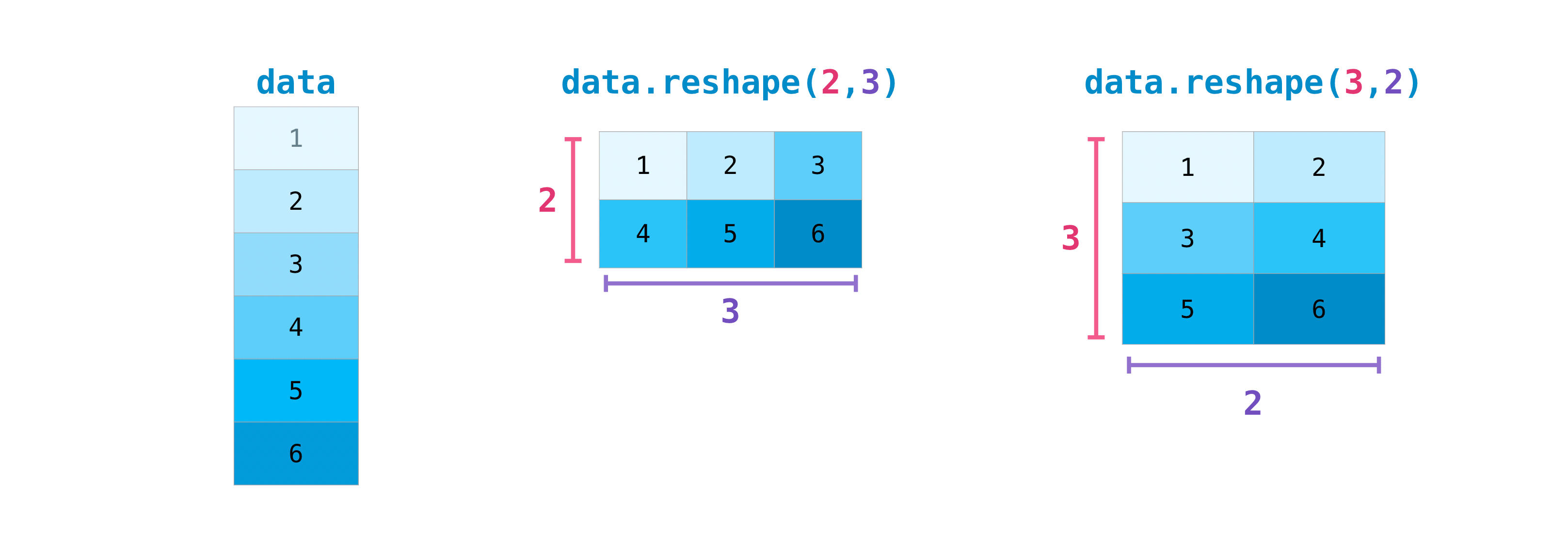
data.reshape(2, 3)

data.reshape(3, 2)

Reversing an array#

NumPy’s np.flip() function allows you to flip, or reverse, the contents of an array along an axis. When using np.flip(), specify the array you would like to reverse and the axis. If you don’t specify the axis, NumPy will reverse the contents along all of the axes of your input array.

Reversing a 1D array

If you begin with a 1D array like this one:

arr = np.array([1, 2, 3, 4, 5, 6, 7, 8])
arr

You can reverse it with:

reversed_arr = np.flip(arr)
reversed_arr

Reversing a 2D array

A 2D array works much the same way.

If you start with this array:

arr_2d = np.array([[1, 2, 3, 4], [5, 6, 7, 8], [9, 10, 11, 12]])
arr_2d

You can reverse the content in all of the rows and all of the columns with:

np.flip(arr_2d)

You can easily reverse only the rows using the axis argument:

np.flip(arr_2d, axis=0)

Or reverse only the columns with:

np.flip(arr_2d, axis=1)

You can also reverse the contents of only one column or row. For example, you can reverse the contents of the row at index position 1 (the second row):

arr_2d[1] = np.flip(arr_2d[1])

arr_2d

You can also reverse the column at index position 1 (the second column):

arr_2d[:,1] = np.flip(arr_2d[:,1])
arr_2d

Converting 1D arrays to 2D (how to add a new axis to an array)#

This section covers np.newaxis, np.expand_dims

You can use np.newaxis and np.expand_dims to increase the dimensions of your existing array.

Using np.newaxis will increase the dimensions of your array by one dimension when used once. This means that a 1D array will become a 2D array, a 2D array will become a 3D array, and so on.

For example, if you start with this array:

a = np.arange(1,7)
a.shape

You can use np.newaxis to add a new axis:

a2 = a[np.newaxis, :]
a2.shape

You can explicitly convert a 1D array to either a row vector or a column vector using np.newaxis. For example, you can convert a 1D array to a row vector by inserting an axis along the first dimension:

row_vector = a[np.newaxis, :]
row_vector.shape

Or, for a column vector, you can insert an axis along the second dimension:

col_vector = a[:, np.newaxis]
col_vector.shape

You can also expand an array by inserting a new axis at a specified position with np.expand_dims.

For example, if you start with this array:

a = np.arange(1, 7)
a.shape

You can use np.expand_dims to add an axis at index position 1 with:

b = np.expand_dims(a, axis=1)
b 

b.shape

You can add an axis at index position 0 with:

c = np.expand_dims(a, axis=0)
c.shape

Find more information about newaxis here and expand_dims here

Reshaping and flattening multidimensional arrays#

There are two popular ways to flatten an array: .flatten() and .ravel(). The primary difference between the two is that the new array created using ravel() is actually a reference to the parent array (i.e., a “view”). This means that any changes to the new array will affect the parent array as well. Since ravel does not create a copy, it’s memory efficient.

If you start with this array:

x = np.array([[1 , 2, 3, 4], [5, 6, 7, 8], [9, 10, 11, 12]])
x

You can use flatten to flatten your array into a 1D array. :

x.flatten()

When you use flatten, changes to your new array will not change the parent array.

For example:

a1 = x.flatten()
a1[0] = 99

a1

x # original

But when you use ravel, the changes you make to the new array will affect the parent array.

For example:

a2 = x.ravel()
a2[0] = 98
a2

x # original has changed!

Generating random numbers#

The use of random number generation is an important part of the configuration and evaluation of many numerical and machine learning algorithms. Whether you need to randomly initialize weights in an artificial neural network, split data into random sets, or randomly shuffle your dataset, being able to generate random numbers (actually, repeatable pseudo-random numbers) is essential.

Numpy provides the np.random module for this type of functionality. This includes functions like:

np.random.integers
np.random.random
np.random.normal
np.random.uniform
np.random.standard_t
and more

Mini-exercise#

Use the documentation for the np.random module to complete the following exercises:

Create a random array of shape (3, 4) with elements between 0 and 1.
Create a random array of 100 elements from a normal distribution with mean 0 and standard deviation 1.
Compute the mean and standard deviation of the random array created in the previous exercise and verify that they are close to the mean and standard deviation you asked for
How does changes in the number of elements in step 2 affect the mean and standard deviation of the random array?
Create a random of array of 100 elements and add it to the array from step 2 and save the result
Take the mean and median of this new array. How does it compare to the mean and median of the array from step 2?

How to save and load NumPy objects#

You will, at some point, want to save your arrays to disk and load them back without having to re-run the code. Fortunately, there are several ways to save and load objects with NumPy. The ndarray objects can be saved to and loaded from the disk files with loadtxt and savetxt functions that handle normal text files, load and save functions that handle NumPy binary files with a .npy file extension, and a savez function that handles NumPy files with a .npz file extension.

The .npy and .npz files store data, shape, dtype, and other information required to reconstruct the ndarray in a way that allows the array to be correctly retrieved, even when the file is on another machine with different architecture.

If you want to store a single ndarray object, store it as a .npy file using np.save. If you want to store more than one ndarray object in a single file, save it as a .npz file using np.savez. You can also save several arrays into a single file in compressed npz format with [savez_compressed]{.title-ref}.

It’s easy to save and load an array with np.save(). Just make sure to specify the array you want to save and a file name. For example, if you create this array:

a = np.array([1, 2, 3, 4, 5, 6])
a

You can save it as “filename.npy” with:

np.save('filename', a)

Check to see if “filename.npy” exists in your JupyterLab or VSCode file explorer! It should exist in the same folder as this notebook.

You can use np.load() to reconstruct your array. :

b = np.load('filename.npy')
b

You can save a NumPy array as a plain text file like a .csv or .txt file with np.savetxt.

csv_arr = np.array([1, 2, 3, 4, 5, 6, 7, 8])

You can easily save it as a .csv file with the name new_file.csv like this:

np.savetxt('new_file.csv', csv_arr)

You can quickly and easily load your saved text file using loadtxt():

np.loadtxt('new_file.csv')

The savetxt() and loadtxt() functions accept additional optional parameters such as header, footer, and delimiter. While text files can be easier for sharing, .npy and .npz files are smaller and faster to read.

You cana more about input output file handling here

Converting mathematical formulas to code#

The ease of implementing mathematical formulas that work on arrays is one of the things that make NumPy so widely used in the scientific Python community.

For example, this is the mean square error formula, the averaged form of the sum of squared errors we discussed last time.

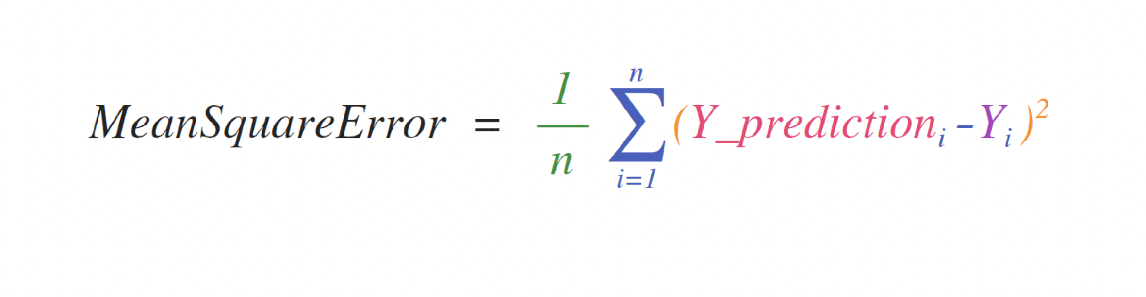
Implementing this formula is simple and straightforward in NumPy:

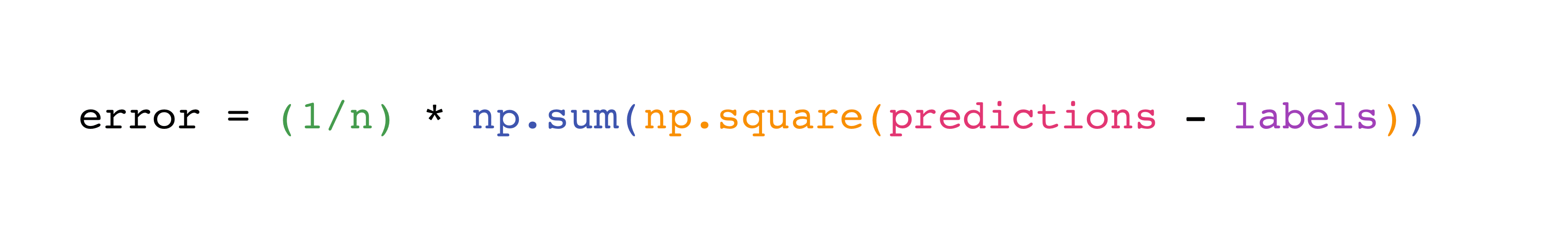
What makes this work so well is that predictions and labels can contain one or a thousand values. They only need to be the same size.

You can visualize it this way:

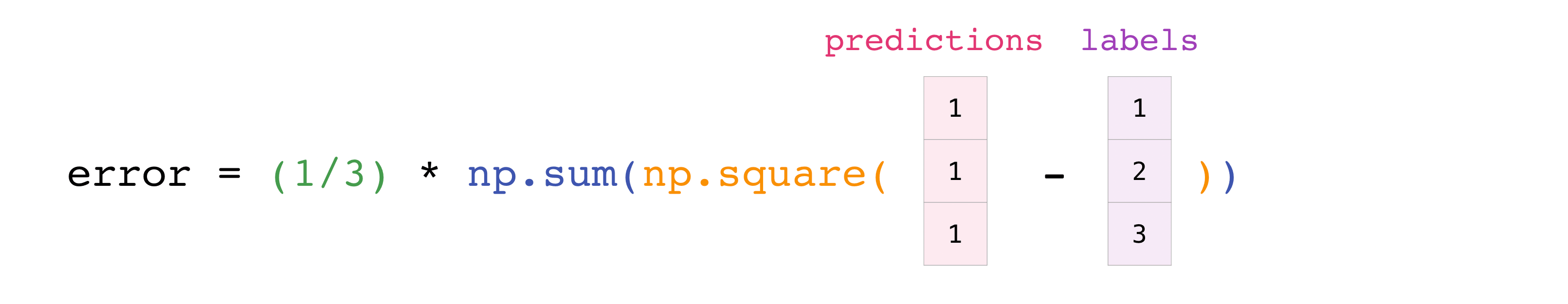
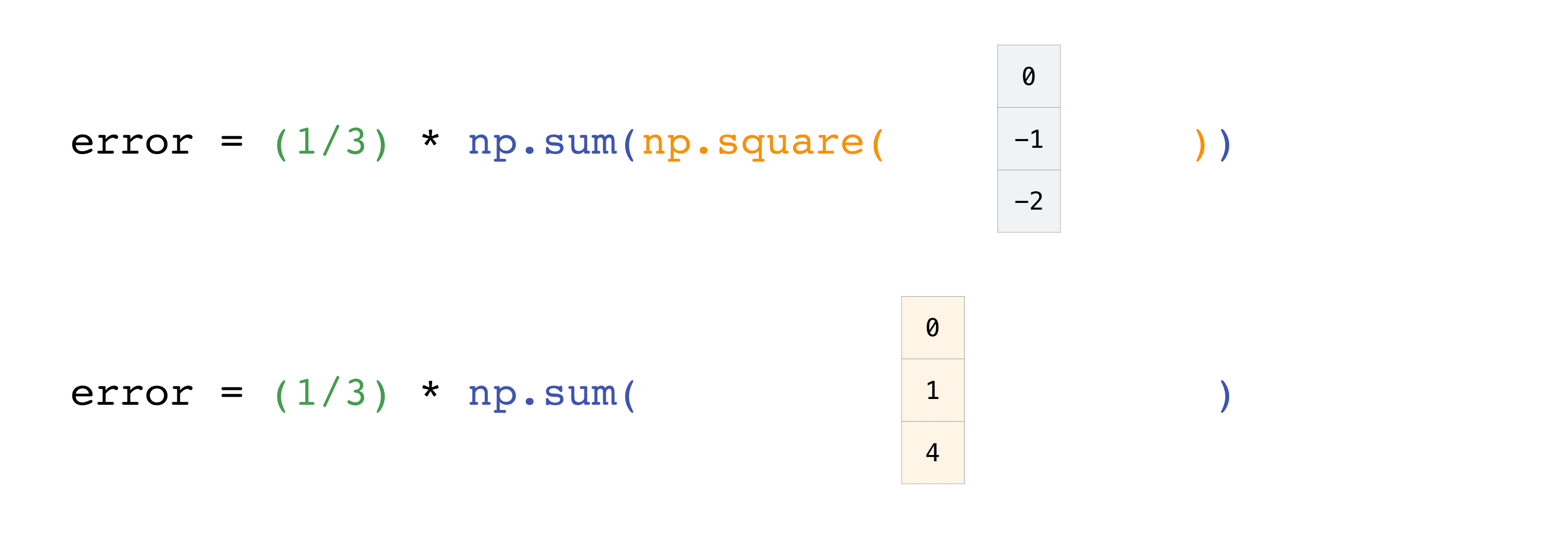
In this example, both the predictions and labels vectors contain three values, meaning n has a value of three. After we carry out subtractions the values in the vector are squared. Then NumPy sums the values, and your result is the error value for that prediction and a score for the quality of the model.

Wrap-up challenge exercise#

We’ve provided a file called image.npy in this folder (you should see it in the file explorer on the left). This is a numpy array containing the RGB values of each pixel in the image.

You can use the imshow() function we’ve imported to display the values of any numpy array, by passing in the array as the first argument (see the setup code-cell below)

Using the notebook and the numpy documentation site try to complete the following tasks:

Create a new array that is the same as the image but flipped vertically (upside down)
Create a new array that is a black-and-white (BW) version of the image; visualize it
Subtract the BW image from the original image; visualize it
Create a new array that adds normally distributed noise to the the black-and-white image; visualize it
Slices the image from steup 4 into a grid of 3 by 3 images; visualize each one
Use the gaussian_filter() function we’ve imported for you, and its linked documentation, apply blur to the image from step 4, and visualize the result

Setup#

import numpy as np
from matplotlib.pyplot import imshow

# Load the image file into a numpy array
img = np.load('image.npy')

# print it's shape
img.shape

Here’s an example of visualizing a NumPy array:

%matplotlib inline
# Visualize the content of the array
# You can add the %matplotlib line to the first line in your code cell in case you don't see the plot
imshow(img)

1. Create a new array that is the same as the image but flipped vertically (upside down)#

2. Create a new array that is a black-and-white (BW) version of the image; visualize it#

3. Subtract the BW image from the original image; visualize it#

4. Create a new array that adds normally distributed noise to the the black-and-white image; visualize it#

5. Slice the image from steup 4 into a grid of 3 by 3 images; visualize each one#

6. Use the `gaussian_filter()` function we’ve imported for you, and its linked documentation, apply blur to the image from step 4, and visualize the result#

from scipy.ndimage import gaussian_filter

image = # your array
blurred = gaussian_filter(image, sigma=2)

Introduction to numpy

Contents

Introduction to numpy#

How to use this notebook#

How to import NumPy#

A note on reading numpy documentation online#

A note on accessing help from within this notebook#

Why use NumPy?#

What is an “array”?#

Array fundamentals#

Arrays vs Lists: Views#

Boolean indexing#

A note on indexing#

A note on terminology#

Array attributes#

Array operations#

Broadcasting#

Note on difference with lists#

More useful array operations#

How to create a basic array#

Specifying your data type#

Creating an array from existing data#

Adding, removing, and sorting elements#

Mini-exercise#

Transposing & Reshaping arrays#

Transposing#

Reshaping#

Reversing an array#

Converting 1D arrays to 2D (how to add a new axis to an array)#

Reshaping and flattening multidimensional arrays#

Generating random numbers#

Mini-exercise#

How to save and load NumPy objects#

Converting mathematical formulas to code#

Wrap-up challenge exercise#

Setup#

1. Create a new array that is the same as the image but flipped vertically (upside down)#

2. Create a new array that is a black-and-white (BW) version of the image; visualize it#

3. Subtract the BW image from the original image; visualize it#

4. Create a new array that adds normally distributed noise to the the black-and-white image; visualize it#

5. Slice the image from steup 4 into a grid of 3 by 3 images; visualize each one#

6. Use the gaussian_filter() function we’ve imported for you, and its linked documentation, apply blur to the image from step 4, and visualize the result#

Introduction to `numpy`#

A note on reading `numpy` documentation online#

6. Use the `gaussian_filter()` function we’ve imported for you, and its linked documentation, apply blur to the image from step 4, and visualize the result#