Models VIII: Multiple Categorical Predictors & ANOVA

Let’s keep working with the poker dataset from the previous notbook and explore models with multiple categorical variables

The experiments used a 2 (skill) x 3 (hand) x 2 (limit) design

Variable	Description
skill	a player’s skill (expert/average)
hand	the quality of the hand experimenters manipulate (bad/neutral/good)
limit	the style of game (fixed/no-limit)
balance	a player’s final balance in Euros

Slides for reference

Modeling VII

import numpy as np
import polars as pl
from polars import col
import seaborn as sns
import matplotlib.pyplot as plt
from statsmodels.formula.api import ols
from statsmodels.stats.anova import anova_lm

# Load data
df = pl.read_csv('./data/poker-tidy.csv')

# Calculate means of each level
bad = df.filter(col('hand') == 'bad')['balance'].mean()
good = df.filter(col('hand') == 'good')['balance'].mean()
neutral = df.filter(col('hand') == 'neutral')['balance'].mean()

means = np.array([bad, good, neutral])

# And the grand-mean
grand_mean = means.mean()

Review: One-way ANOVA

Previously we estimated the model: $\(balance \sim hand\)\( where \)hand\( had 3 levels: \)bad\(, \)neutral\( and \)good$

By using the anova_lm() function we can perform an F-test to see if adding skill to the model is worth it relative to a model with just an intercept. This doesn’t test which levels of skill are different, just whether including skill in the model make a difference in our ability to predict balance.

And we observe that it is: F(2,297) = 75.70, p < .001

one_way = ols('balance ~ C(hand)', data=df.to_pandas())
one_way_results = one_way.fit()

anova_lm(one_way_results, typ=3)

	sum_sq	df	F	PR(>F)
Intercept	3530.142225	1.0	208.830766	3.272007e-36
C(hand)	2559.401402	2.0	75.702581	2.699281e-27
Residual	5020.583223	297.0	NaN	NaN

We also learned that for any categorical predictor with k-levels (k = 3 for hand), we can represent in our GLM represents it using k-1 parameters (2 betas for hand) depending on a variety of coding schemes with different parameter interpretations. And yet all of these yield the same F-test…

The same One-way ANOVA results

1. Treatment (Dummy) Coding

• Default coding scheme

• Intercept = reference level

• Other parameters = differences from reference level

treatment = ols('balance ~ C(hand)', data=df.to_pandas()).fit()
treatment.params

Intercept             5.9415
C(hand)[T.good]       7.0849
C(hand)[T.neutral]    4.4051
dtype: float64

print(f"Intercept = Bad mean {bad:.3f}")
print(f"B1 = Good - Bad {good - bad:.3f}")
print(f"B2 = Neutral - Bad {neutral - bad:.3f}")

Intercept = Bad mean 5.941
B1 = Good - Bad 7.085
B2 = Neutral - Bad 4.405

2. Deviation (Sum) Coding

• Intercept = grand-mean

• Other parameters = differences from grand-mean

sums = ols('balance ~ C(hand, Sum)',data=df.to_pandas()).fit()
sums.params

Intercept               9.7715
C(hand, Sum)[S.bad]    -3.8300
C(hand, Sum)[S.good]    3.2549
dtype: float64

print(f"Intercept = Grand mean {grand_mean:.3f}")
print(f"B1 = Bad - Grand mean {bad - grand_mean:.3f}")
print(f"B2 = Good - Grand mean {good - grand_mean:.3f}")

Intercept = Grand mean 9.771
B1 = Bad - Grand mean -3.830
B2 = Good - Grand mean 3.255

3. Orthogonal (Polynomial) Coding

• Intercept = grand-mean

• Other parameters = trends across levels (e.g. linear, quadratic, cubic)

polys = ols('balance ~ C(hand, Poly)',data=df.to_pandas()).fit()
polys.params

Intercept                  9.771500
C(hand, Poly).Linear       3.114876
C(hand, Poly).Quadratic   -3.986422
dtype: float64

# Approximately the linear contrast Poly uses
lin_con = np.dot([-.707, 0, .707], means)

# Approximately the quadratic contrast Poly uses
quad_con = np.dot([.408, -.816, .408], means)

print(f"Intercept = Grand mean {grand_mean:.3f}")
print(f"Linear contrast = {lin_con:.3f}")
print(f"Quadratic contrast = {quad_con:.3f}")

Intercept = Grand mean 9.771
Linear contrast = 3.114
Quadratic contrast = -3.984

Multiple Categorical Predictors

In the original study the authors also had players of different skill levels participant: \(expert\) and \(average\) players.

Let’s extend our model to test if this additional information is worth adding to our model and whether we need to think more carefully about the coding scheme we’re using…

Let’s do some visual inspection to look at the effects of hand and skill and their interction:

Challenge

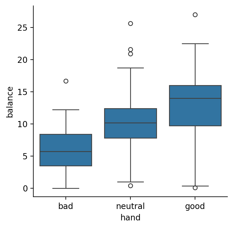
Make 3 boxplot figures all of which plot balance on the y-axis and:

1. hand on the x-axis (“main effect” of hand)

2. skill on the x-axis and on hue (“main effect” of skill)

3. hand on the x-axis and skill on the hue (“interaction” of hand and skill)

1. The effect of hand we estimated in the one-way ANOVA above:

# Solution
grid = sns.catplot(data=df, x='hand', y='balance',kind='box',height=4)

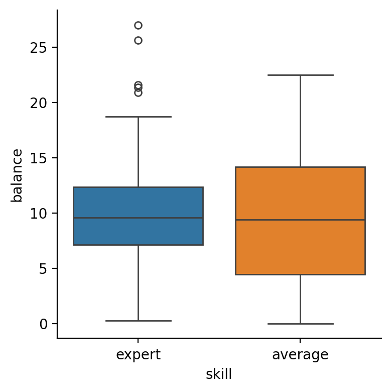
2. The effect of skill

# Solution
grid = sns.catplot(data=df, x='skill', y='balance', hue='skill', kind='box',height=4)

3. The interaction between them, which we can think of as either:

• the difference between skill levels at each level of hand

• the difference between hand levels at each level of skill

# Solution
grid = sns.catplot(data=df, x='hand', y='balance',hue='skill', kind='box', height=4, aspect=1.5)

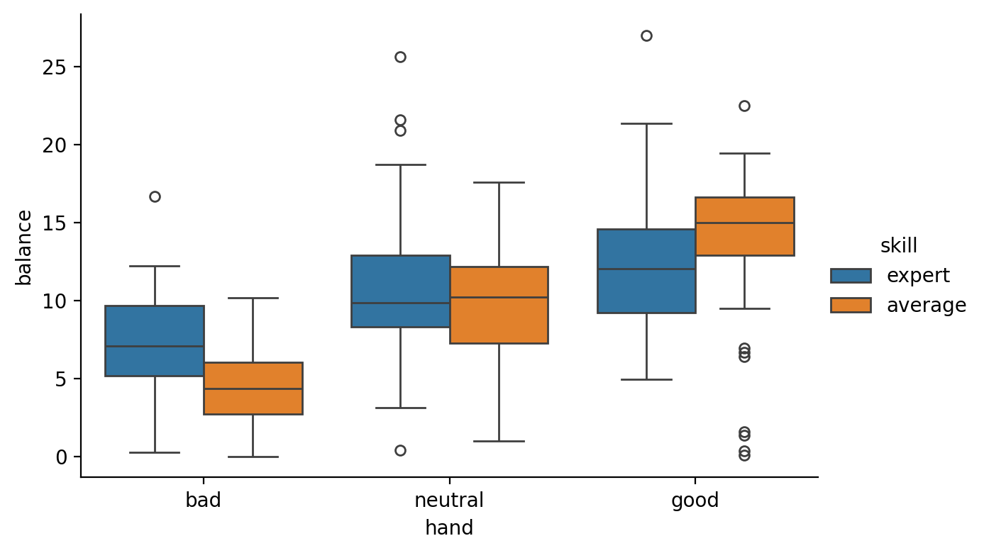
After some visual inspection of the figures it looks like the best way to incorporate additional information about a player’s skill is to estimate a model that includes an interaction between hand and skill. Why? Because it looks like the differences between bad, good, and neutral hands are different for expert vs average players

Challenge

Fit 2 new models that estimate $\(balance \sim hand * skill \)$

• For one of the models using the default treatment coding.

• For the other model use sum coding

Use anova_lm(your_model, type=3) to inspect the F-table for each model separately.

For which model to the results make sense with respect to the figures you made above?

Your response here

# Solution
twoway_treatment = ols('balance ~ C(hand) * C(skill)', data=df.to_pandas()).fit()

anova_lm(twoway_treatment,typ=3).round(4)

	sum_sq	df	F	PR(>F)
Intercept	1051.8450	1.0	65.0728	0.0000
C(hand)	2135.2201	2.0	66.0481	0.0000
C(skill)	183.5754	1.0	11.3570	0.0009
C(hand):C(skill)	228.9817	2.0	7.0830	0.0010
Residual	4752.2521	294.0	NaN	NaN

# Solution
twoway_sums = ols('balance ~ C(hand,Sum) * C(skill, Sum)', data=df.to_pandas()).fit()

anova_lm(twoway_sums, typ=3).round(4)

	sum_sq	df	F	PR(>F)
Intercept	28644.6637	1.0	1772.1137	0.0000
C(hand, Sum)	2559.4014	2.0	79.1692	0.0000
C(skill, Sum)	39.3494	1.0	2.4344	0.1198
C(hand, Sum):C(skill, Sum)	228.9817	2.0	7.0830	0.0010
Residual	4752.2521	294.0	NaN	NaN

Two-way Factorial ANOVA

You should have noticed that using the treatment coding scheme made it seem like the effect of skill was also significant even though \(expert\) and \(average\) players clearly don’t look different from the figure above. So what’s going on?

It turns out that how we code categorical matters for valid F-tests in multiple regression.

In fact this type of multiple regression has a special name, it’s called a factorial ANOVA (analysis of variance).

	Expert	Average
Bad	hand = bad, skill = expert	hand = bad, skill = average
Neutral	hand = neutral, skill = expert	hand = neutral, skill = average
Good	hand = good, skill = expert	hand = good, skill = average

ANOVA is a statistical process initially developed by Ronald Fisher in 1925, for analyzing experiments with only categorical factors. ANOVA provides a mathematical “trick” we can use to efficiently calculate the change in a model’s residual variance attributable to each factor - in the table above the first factor hand had 3 levels and the second factor skill had 2 levels.

ANOVA allows us to decompose this variance to test joint-hypotheses - are all the parameters encoding all the levels of skill (or hand) worth it? For this reason we often refer to an F-test as an omnibus test because it tests all of the parameters encoding a factor at once.

We’ve seen this “change in residual variance” before - it’s the Proportional Reduction in Error (PRE) when we compare nested models! In fact the F-distribution is named in honor of Ronald Fisher - and describes how this change in variance changes as we have more/less factor levels and observations.

However, in order to use this trick and calculate ANOVA correctly there are several key requirements:

• We have to use a valid contrast coding scheme for our categorical variable

• We have to calculate our sum-of-squared residuals using the “type III approach”

There are certain situations in which these conditions won’t matter as much (e.g. perfectly balanced data and factor levels) - but in practice you should follow the guidelines above whenever you plan to conduct F-tests using multiple categorical predictors.

Let’s take a look at each of these now

Valid Contrast coding schemes

You should refer to this week’s reading, especially Chapter 8 of Data Analysis: A Model Comparison Approach, for more additional background details, but in general we consider a categorical coding scheme to be a valid contrast scheme if using values if 2 conditions are met:

• If the codes within each column sum-to-zero

• If overall-sum of codes across columns equals zero

This ensure that our comparisons are orthogonal to each other and yields valid “main effect” and “interaction” F-tests from our ANOVA.

Let’s see the difference between treatment and sum coding:

from helpers import plot_design_matrix

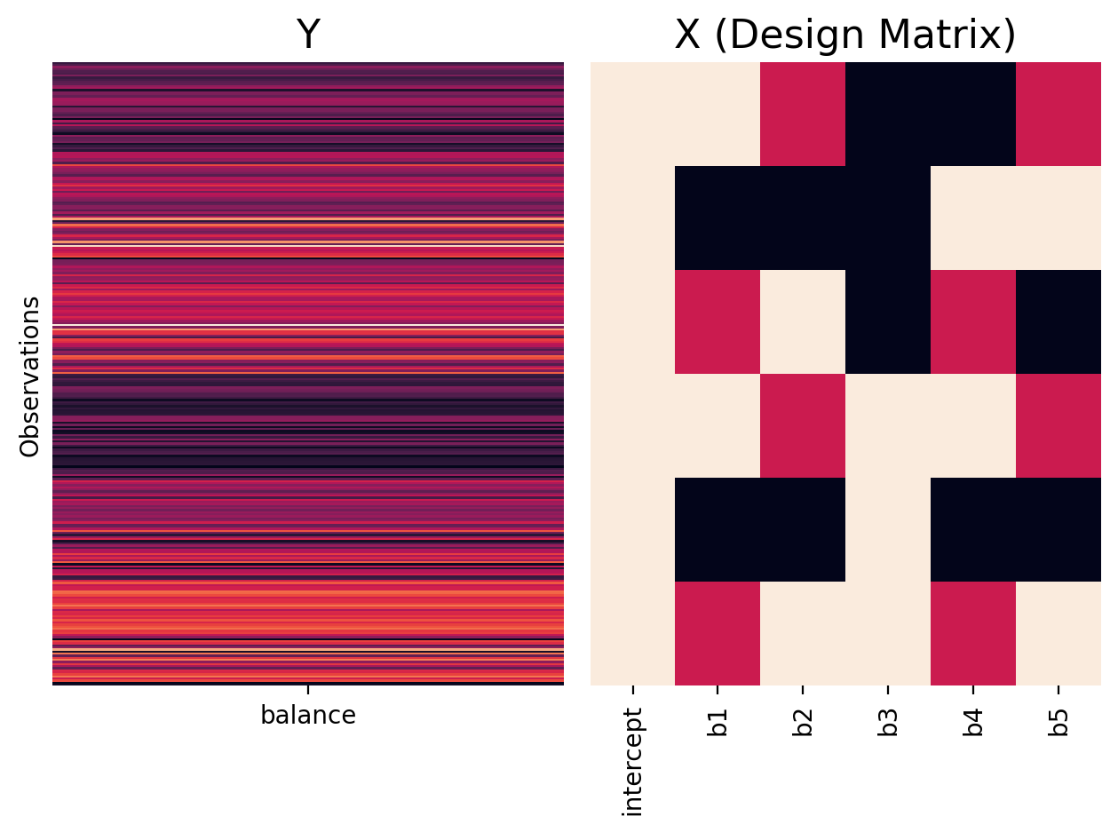
We can see that the treatment/dummy coding using 0s and 1s and therefore doesn’t meet these conditions:

twoway_treatment = ols('balance ~ C(hand) * C(skill)', data=df.to_pandas())
plot_design_matrix(twoway_treatment, plot_names=['intercept','b1','b2','b3','b4','b5'])

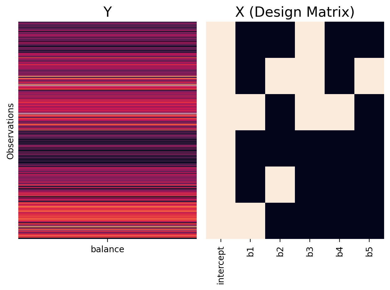
If we add up the rows of our design matrix, ignoring the intercept, our columns do not sum to zero!

twoway_treatment.exog.sum(axis=0)

array([300., 100., 100., 150.,  50.,  50.])

We can also see this by inspecting the coding matrix that ols is using like we did in a previous notebook. This shows the mapping between each level of our categorical predictor and the corresponding reprsentation in the model, like a mini design-matrix.

You can see that it matches the design matrix above (without the intercept)

from patsy.contrasts import Treatment

# All dummy-coded levels of our 2 categorical variables
levels = twoway_treatment.exog_names[1:]

# Generate the coding matrix
treatment_codes = Treatment().code_with_intercept(levels).matrix
treatment_codes

array([[1., 0., 0., 0., 0.],
       [0., 1., 0., 0., 0.],
       [0., 0., 1., 0., 0.],
       [0., 0., 0., 1., 0.],
       [0., 0., 0., 0., 1.]])

And that it fails out first requirement: rows sum-to-zero

treatment_codes.sum(axis=0)

array([1., 1., 1., 1., 1.])

And our second requirement: the overall sum across columns should be zero

treatment_codes.sum(axis=1).sum()

np.float64(5.0)

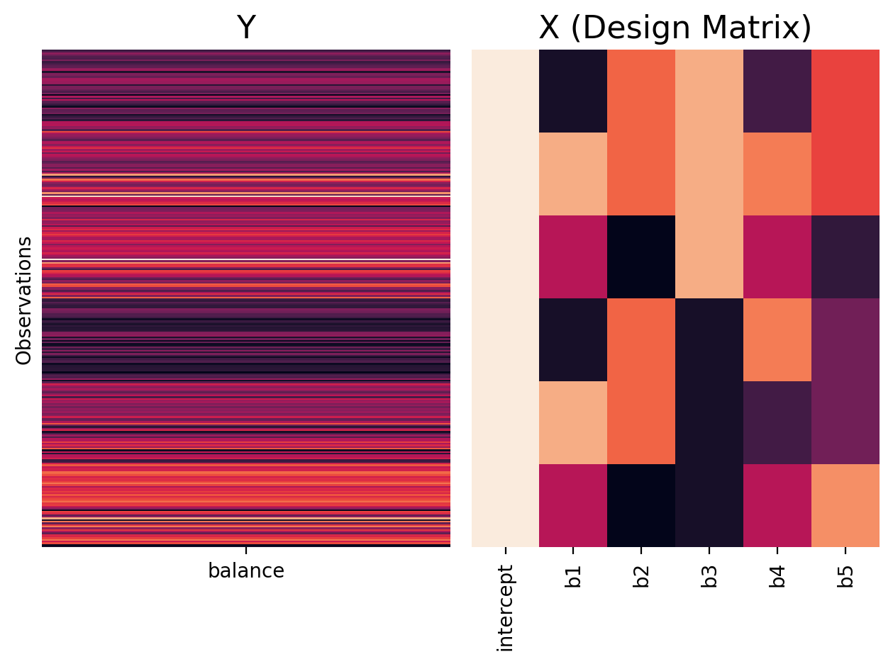
Let’s compare this to deviation/sum coding

twoway_sum = ols('balance ~ C(hand, Sum) * C(skill, Sum)', data=df.to_pandas())
plot_design_matrix(twoway_sum, plot_names=['intercept','b1','b2','b3','b4','b5'])

Again we can check out the model matrix and see it how it maps the different levels of our categorical predictors to numerical values:

from patsy.contrasts import Sum

# All sum-coded levels of our 2 categorical variables
levels = twoway_sum.exog_names[1:]

# Generate the coding matrix
sum_codes = Sum().code_without_intercept(levels).matrix
sum_codes

array([[ 1.,  0.,  0.,  0.],
       [ 0.,  1.,  0.,  0.],
       [ 0.,  0.,  1.,  0.],
       [ 0.,  0.,  0.,  1.],
       [-1., -1., -1., -1.]])

We can see that this scheme is a valid contrast because both rows and sum of columns equal 0:

sum_codes.sum(axis=0)

array([0., 0., 0., 0.])

sum_codes.sum(axis=1).sum()

np.float64(0.0)

Challenge

Using the examples above and the starter code below, can you check if the polynomial scheme is a valid contrast?

Note: often in python you’ll see very small number written using scientific-notation like -2.22044605e-16. For all intent-and-purposes, this is the same as 0 and is due to the way that your computer (and Python) represents the precision of floating-point numbers.

# Define model and plot design matrix here
# Solution
twoway_poly = ols('balance ~ C(hand, Poly) * C(skill, Poly)', data=df.to_pandas())
plot_design_matrix(twoway_poly, plot_names=['intercept','b1','b2','b3','b4','b5'])

# Solution
from patsy.contrasts import Poly

# Fill in with your model's design matrix
levels = twoway_poly.exog_names[1:]

# Generate the coding matrix
poly_codes = Poly().code_without_intercept(levels).matrix

# Your code checking validity here
# Solution
poly_codes.sum(axis=0).round(5)

array([ 0., -0.,  0., -0.])

poly_codes.sum(1).sum().round(5)

np.float64(-0.0)

Type III sums of squares - valid inferences with unbalanced designs

The other requirement for a valid ANOVA is to know what’s refered to as “type III sums of squares.” This isn’t technically a requirement but more of default practice in Psychology and most other social science because of its ability to handle unbalanced designs with interactions.

Fisher’s original formulation of ANOVA assumed that each combination of factor levels had the same number of observations. In experimental terms you might say you have the same \(n\) in each “cell” of your design. When running a factorial ANOVA model with different \(n\) in each cell, the type III method will partition variance for each factor in the way that you expect:

\[\begin{split} SS(A | B, AB)\ \text{for independent variable A} \\ SS(B | A, AB)\ \text{for independent variable B} \\ \end{split}\]

In other words it will calculate the change in model error when adding factor A accounting for both factors B and the interaction between A and B. Intuitively, you can think of this as the same interpretation as when we interpret our parameter estimates: the unique variance of predictor a when accounting for the other predictors b and their interactions a*b.

In other types of SS calculations (I and II) the order in which factors are entered into the model changes the results! This is almost never what you want in practice, so we won’t go into the details of these calculations. Instead you can check out this article for a more detailed explanation with code examples in R.

In your day-to-day work always prefer type III sums-of-squares which you can calculate by making sure to typ=3 with anova_lm

Mini-Exercise

Imagine you were running a replication of the poker study and you didn’t quite get a chance to finish collecting the full set of data. Using the data we’ve loaded for you in the next cell complete the following exercises:

# Load incomplete data
df_inc = pl.read_csv('./data/poker-tidy-incomplete.csv')
df_inc.head()

shape: (5, 4)

skill	hand	limit	balance
str	str	str	f64
"average"	"bad"	"no-limit"	7.84
"expert"	"bad"	"fixed"	8.36
"expert"	"good"	"no-limit"	15.95
"average"	"neutral"	"fixed"	11.89
"expert"	"bad"	"fixed"	11.04

Let’s just focus on the skill and hand variables. How many observations per cell of the design in these data? And how does this compare to the original data (df variable)?

# Solution
df_inc.group_by(['hand','skill']).len()

shape: (6, 3)

hand	skill	len
str	str	u32
"neutral"	"expert"	37
"bad"	"expert"	44
"bad"	"average"	42
"good"	"average"	38
"neutral"	"average"	39
"good"	"expert"	40

# Solution
df.group_by(['hand','skill']).len()

shape: (6, 3)

hand	skill	len
str	str	u32
"bad"	"expert"	50
"neutral"	"average"	50
"bad"	"average"	50
"neutral"	"expert"	50
"good"	"expert"	50
"good"	"average"	50

Below we’ve estimated a model with the same predictors hand and skill, input to the model in two different orders. For some reason the F-statistics and mean_sq (error) of each factor are different between the models.

Can you figure out why? What can you change so that the order doesn’t matter?

We need to use type 3 sums of squares

hand_skill_treatment = ols('balance ~ C(hand) + C(skill)', data=df_inc.to_pandas()).fit()
anova_lm(hand_skill_treatment, typ=1).round(4)

	df	sum_sq	mean_sq	F	PR(>F)
C(hand)	2.0	1972.7168	986.3584	59.4160	0.0000
C(skill)	1.0	22.9502	22.9502	1.3825	0.2409
Residual	236.0	3917.8128	16.6009	NaN	NaN

skill_hand_treatment = ols('balance ~ C(skill) + C(hand)', data=df_inc.to_pandas()).fit()
anova_lm(skill_hand_treatment, typ=1).round(4)

	df	sum_sq	mean_sq	F	PR(>F)
C(skill)	1.0	21.2849	21.2849	1.2822	0.2586
C(hand)	2.0	1974.3820	987.1910	59.4661	0.0000
Residual	236.0	3917.8128	16.6009	NaN	NaN

# Solution
anova_lm(hand_skill_treatment, typ=3)

	sum_sq	df	F	PR(>F)
Intercept	1968.384433	1.0	118.570935	1.224542e-22
C(hand)	1974.382034	2.0	59.466108	1.220272e-21
C(skill)	22.950190	1.0	1.382466	2.408662e-01
Residual	3917.812805	236.0	NaN	NaN

# Solution
anova_lm(skill_hand_treatment, typ=3)

	sum_sq	df	F	PR(>F)
Intercept	1968.384433	1.0	118.570935	1.224542e-22
C(skill)	22.950190	1.0	1.382466	2.408662e-01
C(hand)	1974.382034	2.0	59.466108	1.220272e-21
Residual	3917.812805	236.0	NaN	NaN

Looking back at either model, it turns out we may not actually be calculating a valid ANOVA based on our coding scheme…

Fit a new model that estimates a valid ANOVA. Compare the F statistics of this model and the previous two models. What do you notice?

*The F-stat for hand matches skill_hand_treatment and the F-stat for skill matches hand_skill_treatment because type I SS is sequential so it first accounts for variance from the first entered term before calculating remaining variance for the second. Type III does this automatically, calculating unique variance for each factor irrespective of order!

# Solution
skill_hand_sum = ols('balance ~ C(skill,Sum) + C(hand,Sum)', data=df_inc.to_pandas()).fit()
anova_lm(skill_hand_treatment, typ=3).round(4)

	sum_sq	df	F	PR(>F)
Intercept	1968.3844	1.0	118.5709	0.0000
C(skill)	22.9502	1.0	1.3825	0.2409
C(hand)	1974.3820	2.0	59.4661	0.0000
Residual	3917.8128	236.0	NaN	NaN

Additional Coding Systems for Categorical Variables

We’ve only been focusing on the 3 most common coding schemes that you’ll use in practice:

• treatment (not valid for ANOVA)

• deviation (valid for ANOVA)

• polynomial (valid for ANOVA)

Below we’ve linked to a few other resources that cover additional coding schemes that you may consider in practice.

• Coding Systems for Categorical Variables conceptual overview, but examples are in R

• Contrasts in StatsModels Shorter Python version of the guide above

• How to use different coding schemes in formulas

In a later notebook we’ll explore how to parameterize our model to test specific planned comparisons and to follow up an estimate with additional post-hoc comparisons