Common Formulas#
Note
This page contains formulas for statistical quantities we’ve discussed so far. We’ll add more as we go along.
# NumPy for basic statistics and linear algebra
import numpy as np
Summarizing single variables#
Mode#
Definition: The most common value in the data
mode = np.mode(data)
Median#
Definition: The middle value after sorting the data from lowest to highest - or the average of middle values if there is an even number of data points
Intuition: A simple summary “model” of the data that minimizes the the sum of absolute errors - i.e. the absolute distance of each data point from the median
median = np.median(data)
Mean#
Definition: The average of all the data points - often called the expected value in other settings
Intuition: A simple summary “model” of the data that minimizes the the sum of squared errors - i.e. the squared distance of each data point from the mean
mean = np.mean(data)
Variance#
Definition: The average of the squared distance of each data point from the mean; we use \(n-1\) instead of \(n\) to account for the sample mean \(\bar{x}\) that we depend upon
Intuition v1: How dispersed the data are around the mean
Intuition v2: The average prediction-error of the mean as a model for the data
variance = np.var(data)
Standard Deviation#
Definition: The square root of the variance
Intuition: Variance in units of standardized distance from the mean
std_dev = np.std(data)
Z-Score#
Definition: The standardized distance of each data point from the mean by subtracting the mean and dividing by standard deviation
Intuition: Centering and scaling the data into units of “standardized distance from the mean” to make data comparable across different measurement scales
# Easiest
from scipy.stats import zscore

z_scores = zscore(data)

# Manually
z_scores = (data - np.mean(data)) / np.std(data)

# Or if data is an array you can use method, i.e. "." syntax
z_scores = (data - data.mean()) / data.std()
Vector Norm#
Definition: Square-root of the sum of each element squared
Intuition: Reflects the magnitude/length of a vector of data, specifically in terms of how far it is from 0 (the origin). If variance is average spread of the data around the mean, the norm is the total spread of the data (distance) from the value 0.
Linear algebra style:
# Easiest
norm = np.linalg.norm(x)

# Manually:
norm = np.sqrt(np.sum(x**2))

# linear algebra style
norm = np.sqrt(np.dot(x.T, x))
Summarizing relationships#
Dot Product#
Definition: Sum of the products of each pair of elements
Intuition: If x and y “move together” the dot-product will be higher - but sensitive to the units of the measurement
dot_product = np.dot(x, y)

# Manually
np.sum(x * y)
Cosine Similarity#
Definition: Dot product normalized, i.e. divided by, the product of vector norms
Intuition: Scale the dot-product to standardized units of “distance from 0” - no longer sensitive to the units of the measurement and bounded between -1 and 1
# X norm - manually
x_norm = np.sqrt(np.sum(x**2))

# Y norm - easier just use numpy
y_norm = np.linalg.norm(y)

# Scale dot product to standardized units of "*distance from 0*"
cosine_similarity = np.dot(x, y) / (x_norm * y_norm)

# OR
from scipy.spatial.distance import cosine

# Convert distance to similarity using 1-cosine
cosine_similarity = 1 - cosine(x, y)
Average Dot/Inner Product#
Definition: Just divide dot-product by the number of elements
Intuition: Behaves just like the dot-product, but scale is more intuitive to understand - still sensitive to the units of the measurement
avg_dot_product = np.dot(x, y) / len(x)
Covariance#
Definition: Mean-centered average dot-product - use \(n-1\) instead of \(n\) to account for the sample mean(s) we depend upon
Intuition: Measure how much x and y “move together” around their respective means; “anchors” the average dot product to the centers (means) of each variable - still sensitive to the units of measurement
covariance = np.dot(x - x.mean(), y - y.mean()) / (len(x) - 1)

# OR
# Returns 2d array: off-diagonals are covariance; diagonals are variances
covariance = np.cov(x, y)
Pearson Correlation#
Intuition: Measure how much x and y “move together” around their respective means - in units of standardized distance from the mean - i.e. z-scores - best used when you want to detect linear relationships
Definition v1: Covariance normalized by product of standard deviations
correlation = covariance / np.std(x) * np.std(y)
Definition v2: Average dot-product of z-scores
from scipy.stats import zscore

z_x = zscore(x)
z_y = zscore(y)

correlation = np.dot(z_x, z_y) / (len(x) - 1)
Useful functions in practice:
# Scipy
from scipy.stats import pearsonr
result = pearsonr(x, y)

result.statistic # correlation
result.pvalue # p-value
result.confidence_interval # 95% confidence interval

# Numpy
# Off-diagonals are correlation
correlation_matrix = np.corrcoef(x, y)

# Or as single array
2d_xy = np.vstack([x,y])
correlation_matrix = np.corrcoef(2d_xy)
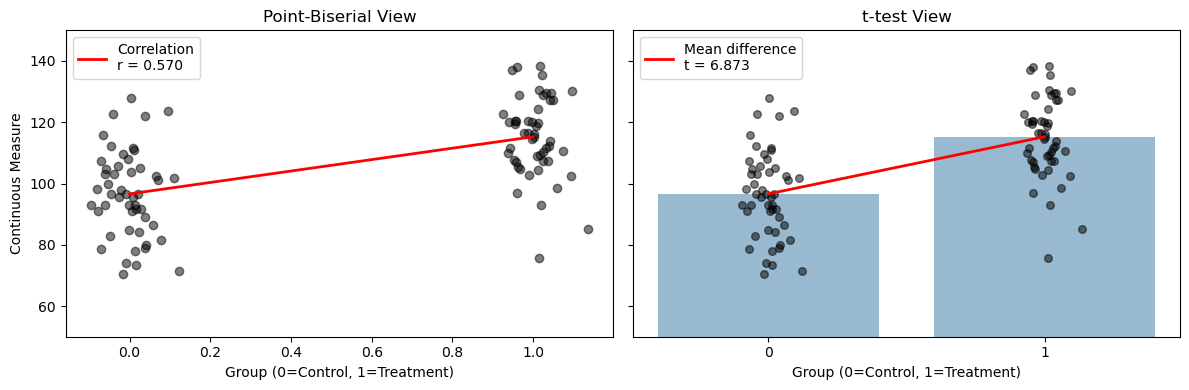
Point-Biserial Correlation (Special Case)#
Definition: Point-biserial correlation is a special case of Pearson’s correlation used when one variable is binary (e.g., 0/1, False/True) and the other is continuous.
Intuition: When one of your variables is binary, the correlation is akin to a test of the difference between two means, i.e. an indepdendent samples t-test.
from scipy.stats import pointbiserialr

result = pointbiserialr(x_binary, y)

# Equivalent to:
from scipy.stats import pearsonr
result = pearsonr(x_binary, y)
In fact you can convert between the point biserial \(r\) and the student’s \(t\) using the following formulas:
from scipy.stats import ttest_ind, pointbiserialr # or pearsonr

r_result = pointbiserialr(x_binary, y)
r = r_result.statistic

# Make groups using boolean indexing
group_a = y[x_binary == 0]
group_b = y[x_binary == 1]

t_result = ttest_ind(group_a, group_b)
t = t_result.statistic

#  r -> t
t_from_r = r * np.sqrt( (len(binary) - 2) / (1 - r**2))

# t -> r
r_from_t = t / np.sqrt(t**2 + (len(binary) - 2))

# True
t == t_from_r
r == r_from_t
Spearman (Rank) Correlation#
Definition: Transform data to ranks and then calculate Pearson correlation on the ranks
Intuition: Whereas a Pearson correlation assumes that both variables move at a constant rate with respect to each other (linear relationship), Spearman correlation only assumes that the order of both variables move together at a constant rate (monotonic relationship).
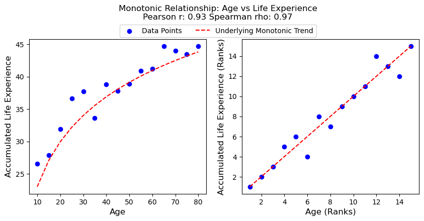
In other words, both variables must move together in the same direction (increasing or decreasing) but not necessarily at the same rate. For example, a person’s age and their accumulated life experience have a monotonic relationship. As a person gets older, their life experience tends to not only increase, but increase at a different rate than how age increases over their lifetime.
Rank-transforming them will normalize these different rates of change into units of “rank-change” - making Spearman correlation more sensitive than Pearson correlation in situations of skewed distributions or outliers.
# Rank the data
from scipy.stats import rankdata
x_ranks = rankdata(x)
y_ranks = rankdata(y)

# Compute Pearson correlation on ranked data
results = pearsonr(x_ranks, y_ranks)

# In practice just use spearmanr directly:
from scipy.stats import spearmanr

results = spearmanr(x, y)
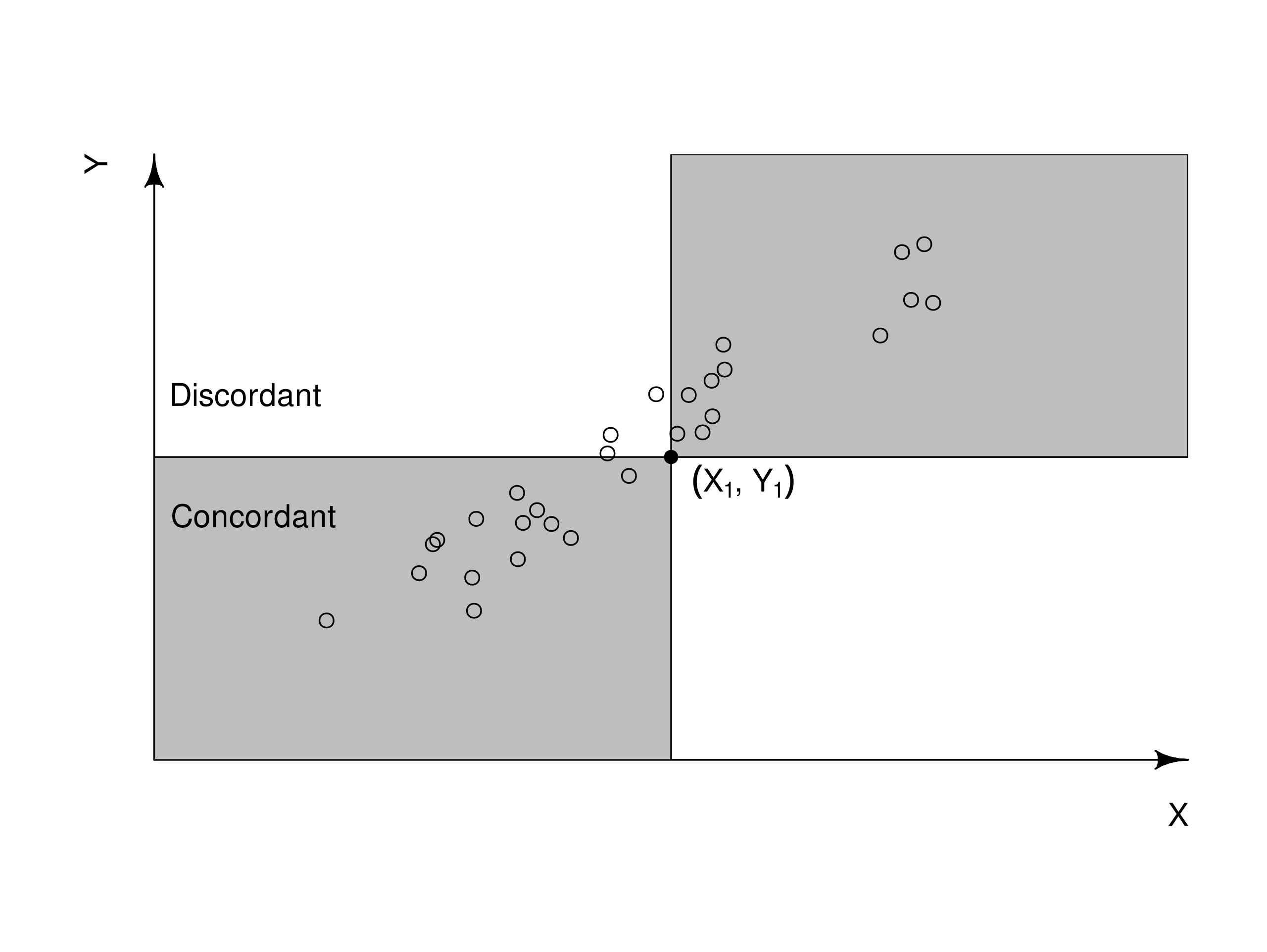
Kendall’s Tau (Rank)#
Definition: Count the proportion of \((x,y)\) pairs that are concordant vs discordant
Intuition: Also works with ranks and measures monotonicity by literally counting up pairs of \((x,y)\) that increase/decrease together (concordant) vs those that don’t (discordant). It’s particularly useful when dealing with small datasets or when rank-transforming produces lots of tied rankings.
from scipy.stats import kendalltau

result = kendalltau(x, y)