Models IX: ANOVA and additional comparisons#
Note:
Before running this notebook open a terminal, activate the 201b environment, and install the marginaleffects package:
Open terminal
conda activate 201bpip install marginaleffects
Let’s keep working with the poker dataset from the previous notebook and explore models how we can ask additional questions about the data
The experiments used a 2 (skill) x 3 (hand) x 2 (limit) design
Variable |
Description |
|---|---|
skill |
a player’s skill (expert/average) |
hand |
the quality of the hand experimenters manipulate (bad/neutral/good) |
limit |
the style of game (fixed/no-limit) |
balance |
a player’s final balance in Euros |
Slides for reference
Let’s start by loading the data, plotting the interaction effect of hand and skill on balance, and estimating our valid two-way ANOVA
import numpy as np
import polars as pl
from polars import col
from polars import when, lit
import seaborn as sns
import matplotlib.pyplot as plt
from statsmodels.formula.api import ols
from statsmodels.stats.anova import anova_lm

# Load data
df = pl.read_csv('./data/poker-tidy.csv')
# Sum code our categorical variables because sum coding is a valid contrast for ANOVA
model = ols("balance ~ C(hand, Sum) * C(skill, Sum)", data=df.to_pandas())

# Estimate model
results = model.fit()
# Use type III SS to calculate F-stats for main effects and interactions
anova_lm(results, typ=3).round(4)
| sum_sq | df | F | PR(>F) | |
|---|---|---|---|---|
| Intercept | 28644.6637 | 1.0 | 1772.1137 | 0.0000 |
| C(hand, Sum) | 2559.4014 | 2.0 | 79.1692 | 0.0000 |
| C(skill, Sum) | 39.3494 | 1.0 | 2.4344 | 0.1198 |
| C(hand, Sum):C(skill, Sum) | 228.9817 | 2.0 | 7.0830 | 0.0010 |
| Residual | 4752.2521 | 294.0 | NaN | NaN |
Unpacking the ANOVA#
Whenever we’re running an ANOVA we need to make a distinction between main effects and simple effects that doesn’t come up when we’re using continuous predictors. Remember that the F-tests in the output above are omnibus or joint-tests - they tell us whether factor as a whole matters, not which specific factor levels are different:
main effect: effect of entire independent variable (IV) e.g.
handon dependent variable (DV)interaction effect: when the main effect of one IV depends upon the levels of another IV e.g.
skillsimple effect: comparisons between specific levels of an IV - i.e. “cell means” comparisons, e.g.
goodvsbadwithinhand
Above we see a significant interaction which we can interpret as differences between differences:
the difference between levels of
handare different across levels ofskillOR the difference between levels of
skillare different across levels ofhand
But what specific differences? Let’s explore two ways we can test more specific hypotheses:
“Post-hoc” pairwise cell-mean comparisons#
The simplest approach we can take is to use “post-hoc” pairwise comparisons. We say this is post-hoc because we’re testing additional hypotheses after our main model.
The most common way to do this is to perform “pairwise” comparisons: comparisons between every pair of cell means, i.e. every combination of levels of the two factors:
# Calculate cell means for each combination of factor levels
cell_means = df.group_by(['hand','skill']).agg(
    col('balance').mean()).sort(['hand','skill'])

cell_means
| hand | skill | balance |
|---|---|---|
| str | str | f64 |
| "bad" | "average" | 4.5866 |
| "bad" | "expert" | 7.2964 |
| "good" | "average" | 13.7976 |
| "good" | "expert" | 12.2552 |
| "neutral" | "average" | 9.8438 |
| "neutral" | "expert" | 10.8494 |
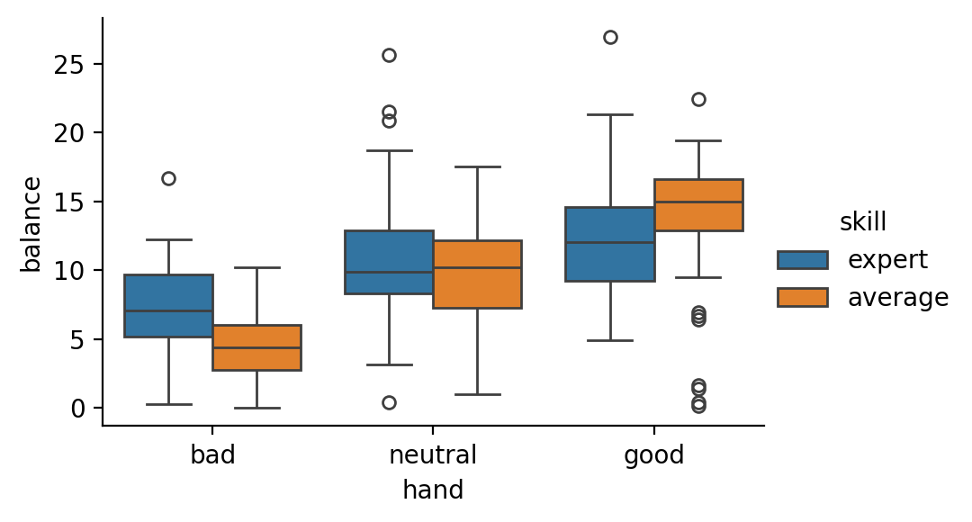
Visually, you can think about that as directly comparing each individual box in the boxplot above to every other box
# Our box plot shows the mean of each cell
grid = sns.catplot(data=df, x='hand', y='balance',hue='skill', kind='box', height=3, aspect=1.5)
Because these comparisons are no longer independent, we have to adjust our alpha level which - raise the threshold at which we decide to reject the null hypothesis based upon our p-value. In other words decrease, our typical threshold of p < .05 where alpha = .05 to p < new_alpha, where new_alpha is something smaller than .05.
This idea, called multiple comparisons correction, comes in may flavors with the same underlying goal: reduce the number of false positive results we find while minimizing the number of false negative results we don’t find.
Three of the most common approaches from most to least strict (in terms of false positives at the expense of false negatives):
Bonferroni =
alpha / n- we just adjust our p-value threshold to smaller for each comparison we run1 test: alpha = .05
2 tests: alpha = .05 / 2 = .025
3 tests: alpha = .05 / 3 = .0167
Most conservative (fewest false positives); but also most stringent (most false negatives)
Holm-Bonferroni = “sequential” bonferroni - we adjust our p-value threshold to smaller for each comparison we run, but we also adjust the threshold for the next comparison to be smaller than the previous one
Much better balanced than Bonferroni when we have lots of comparisons to make
False discovery rate (FDR) - we adjust our alpha threshold based upon the size of our p-values, such that we apply Bonferroni correction to the smallest p-value we find and apply a less stringest correction for the next smallest p-value, etc
Ideal when the number of comparisons is very large; but also increases false positive rate
Instructor’s Note#
Performing custom cell mean comparisons are a bit easier in R thanks to the emmeans package, which doesn’t have a perfect counter-part in Python 😢.
In one more week, when we discuss repeated-measures/multi-level models (lmer in R), things will get a bit easier because we’ll use a Python package that does supports emmeans like functionality.
For now, we’ll show you a few different ways perform these comparisons in Python, each with their own pros and cons.
Within factor comparisions using statsmodels#
Main approach:
Use
.t_test_pairwise()method on the results of your model (i.e. the output of.fit())
Pros
No additional libraries needed
Straightforward to use
Built-in support for multiple comparisons correction
Cons
Need to name variables exactly like they are in your model’s formula
Can only compare levels within a factor, i.e. no interactions!
Can’t get cell means easily
The first argument to the method is the name of first predictor exactly like it appears in our model formula, and the method argument provides support for a variety of multiple comparisons corrections. In our data here, we don’t have that many comparisons and the differences are so large that our multiple-comparisons correction method doesn’t really matter
# Pairwise differences of levels of hand
results.t_test_pairwise("C(hand, Sum)", method='bonferroni').result_frame
| coef | std err | t | P>|t| | Conf. Int. Low | Conf. Int. Upp. | pvalue-bonferroni | reject-bonferroni | |
|---|---|---|---|---|---|---|---|---|
| good-bad | 7.0849 | 0.568579 | 12.460706 | 6.667347e-29 | 5.965899 | 8.203901 | 2.000204e-28 | True |
| neutral-bad | 4.4051 | 0.568579 | 7.747556 | 1.530999e-13 | 3.286099 | 5.524101 | 4.592996e-13 | True |
| neutral-good | -2.6798 | 0.568579 | -4.713151 | 3.769889e-06 | -3.798801 | -1.560799 | 1.130967e-05 | True |
# Same thing but with a more liberal correction method
results.t_test_pairwise("C(hand, Sum)", method='fdr_bh').result_frame
| coef | std err | t | P>|t| | Conf. Int. Low | Conf. Int. Upp. | pvalue-fdr_bh | reject-fdr_bh | |
|---|---|---|---|---|---|---|---|---|
| good-bad | 7.0849 | 0.568579 | 12.460706 | 6.667347e-29 | 5.965899 | 8.203901 | 2.000204e-28 | True |
| neutral-bad | 4.4051 | 0.568579 | 7.747556 | 1.530999e-13 | 3.286099 | 5.524101 | 2.296498e-13 | True |
| neutral-good | -2.6798 | 0.568579 | -4.713151 | 3.769889e-06 | -3.798801 | -1.560799 | 3.769889e-06 | True |
Challenge (mini)#
Using the two examples above, use .t_test_pairwise() to compute the diffence between levels of skill
Using the original dataframe df, verify that the value in the coef column is indeed the difference between the two levels of skill.
# Your code here
# Solution
results.t_test_pairwise("C(skill, Sum)").result_frame
| coef | std err | t | P>|t| | Conf. Int. Low | Conf. Int. Upp. | pvalue-hs | reject-hs | |
|---|---|---|---|---|---|---|---|---|
| expert-average | 0.724333 | 0.464243 | 1.560246 | 0.119778 | -0.189328 | 1.637994 | 0.119778 | False |
With marginaleffects library#
marginaleffects is a very neat library that supports both R and Python and can handle a lot of different types of marginal comparisons and estimates. Unfortunately, the Python version doesn’t yet have all the features of the R version.
However, it’s useful precisely because the previous approach using .t_test_pairwise doesn’t handle comparisons between cell means across different factor levels, but marginaleffects does!
Main approach:
avg_predictions()function for cell meansavg_predictions()function with thehypothesisargument for pairwise comparisons
Pros
Can refer to variables based on their column names
Easy to get cell means and comparisons
Supports interaction and complex pairwise comparisons (e.g. with continuous predictors)
Support many other types of analyses
Has a comparable R package
Cons
Doesn’t support multiple comparisons correction
Commands (syntax) can be a little wonky
Not all R-version features are supported in Python
We can use the marginaleffects package which takes our estimated model results as input and a by argument that is one of our predictor variables as named in our dataframe:
Marginal means of each level of hand (averaged across skill)
from marginaleffects import avg_predictions

avg_predictions(results, by='hand')
| hand | estimate | std_error | statistic | p_value | s_value | conf_low | conf_high |
|---|---|---|---|---|---|---|---|
| str | f64 | f64 | f64 | f64 | f64 | f64 | f64 |
| "bad" | 5.9415 | 0.402046 | 14.778146 | 0.0 | inf | 5.153504 | 6.729496 |
| "good" | 13.0264 | 0.402047 | 32.40023 | 0.0 | inf | 12.238403 | 13.814397 |
| "neutral" | 10.3466 | 0.402046 | 25.734846 | 0.0 | inf | 9.558604 | 11.134596 |
Marginal means of each level of skill (averaged across hand)
avg_predictions(results, by='skill')
| skill | estimate | std_error | statistic | p_value | s_value | conf_low | conf_high |
|---|---|---|---|---|---|---|---|
| str | f64 | f64 | f64 | f64 | f64 | f64 | f64 |
| "average" | 9.409333 | 0.32827 | 28.66342 | 0.0 | inf | 8.765936 | 10.05273 |
| "expert" | 10.133667 | 0.32827 | 30.869944 | 0.0 | inf | 9.49027 | 10.777063 |
We can get the individual cell means (combinations of factor levels) by passing a list to by:
avg_predictions(results, by=['hand','skill'])
| hand | skill | estimate | std_error | statistic | p_value | s_value | conf_low | conf_high |
|---|---|---|---|---|---|---|---|---|
| str | str | f64 | f64 | f64 | f64 | f64 | f64 | f64 |
| "bad" | "average" | 4.5866 | 0.568579 | 8.066772 | 6.6613e-16 | 50.415037 | 3.472205 | 5.700995 |
| "bad" | "expert" | 7.2964 | 0.568579 | 12.832684 | 0.0 | inf | 6.182005 | 8.410795 |
| "good" | "average" | 13.7976 | 0.568579 | 24.266791 | 0.0 | inf | 12.683205 | 14.911995 |
| "good" | "expert" | 12.2552 | 0.568579 | 21.554067 | 0.0 | inf | 11.140805 | 13.369595 |
| "neutral" | "average" | 9.8438 | 0.568579 | 17.312975 | 0.0 | inf | 8.729405 | 10.958195 |
| "neutral" | "expert" | 10.8494 | 0.568579 | 19.081592 | 0.0 | inf | 9.735005 | 11.963795 |
We can also add the hypothesis = 'pairwise' argument to any of the same commands above to calculate differences between the calculate marginal or cell means.
Marginal mean differences within levels of hand
avg_predictions(results, by='hand', hypothesis='pairwise')
| term | estimate | std_error | statistic | p_value | s_value | conf_low | conf_high |
|---|---|---|---|---|---|---|---|
| str | f64 | f64 | f64 | f64 | f64 | f64 | f64 |
| "bad - good" | -7.0849 | 0.56858 | -12.4607 | 0.0 | inf | -8.199296 | -5.970504 |
| "bad - neutral" | -4.4051 | 0.568579 | -7.747554 | 9.3259e-15 | 46.607683 | -5.519495 | -3.290705 |
| "good - neutral" | 2.6798 | 0.56858 | 4.713149 | 0.000002 | 18.645174 | 1.565405 | 3.794195 |
Marginal mean differences within levels of skill
avg_predictions(results, by='skill', hypothesis='pairwise')
| term | estimate | std_error | statistic | p_value | s_value | conf_low | conf_high |
|---|---|---|---|---|---|---|---|
| str | f64 | f64 | f64 | f64 | f64 | f64 | f64 |
| "average - expert" | -0.724333 | 0.464244 | -1.560243 | 0.118702 | 3.074579 | -1.634234 | 0.185568 |
And by passing a list to by again along with hypothesis we can get the pairwise comparison between each combination of factor levels
Since we have 3 levels of hand (bad, good, neutral) and 2 levels of skill (expert, average) we have 6 unique combinations of factor levels to compare
The unique number of pairs is \(n*(n-1)/2\) or in our case \(6*5/2=15\)
all_pairs = avg_predictions(results, by=['hand','skill'], hypothesis='pairwise')

all_pairs.height
15
all_pairs
| term | estimate | std_error | statistic | p_value | s_value | conf_low | conf_high |
|---|---|---|---|---|---|---|---|
| str | f64 | f64 | f64 | f64 | f64 | f64 | f64 |
| "bad, average - bad, expert" | -2.7098 | 0.804093 | -3.370009 | 0.000752 | 10.377639 | -4.285793 | -1.133807 |
| "bad, average - good, average" | -9.211 | 0.804093 | -11.455149 | 0.0 | inf | -10.786992 | -7.635008 |
| "bad, average - good, expert" | -7.6686 | 0.804093 | -9.536958 | 0.0 | inf | -9.244593 | -6.092607 |
| "bad, average - neutral, averag… | -5.2572 | 0.804093 | -6.538053 | 6.2325e-11 | 33.901402 | -6.833192 | -3.681208 |
| "bad, average - neutral, expert" | -6.2628 | 0.804093 | -7.788653 | 6.8834e-15 | 47.045804 | -7.838793 | -4.686807 |
| … | … | … | … | … | … | … | … |
| "good, average - neutral, avera… | 3.9538 | 0.804092 | 4.917096 | 8.7837e-7 | 20.118663 | 2.377808 | 5.529792 |
| "good, average - neutral, exper… | 2.9482 | 0.804093 | 3.666491 | 0.000246 | 11.989632 | 1.372207 | 4.524193 |
| "good, expert - neutral, averag… | 2.4114 | 0.804093 | 2.998907 | 0.002709 | 8.527759 | 0.835407 | 3.987393 |
| "good, expert - neutral, expert" | 1.4058 | 0.804093 | 1.748306 | 0.080411 | 3.636463 | -0.170193 | 2.981793 |
| "neutral, average - neutral, ex… | -1.0056 | 0.804093 | -1.250602 | 0.21108 | 2.24414 | -2.581593 | 0.570393 |
Because the comparison names can get lengthy we can just pull them out into a list using normal polars commands:
# Names are little easier to read
all_pairs[:, 0].to_list()
['bad, average - bad, expert',
 'bad, average - good, average',
 'bad, average - good, expert',
 'bad, average - neutral, average',
 'bad, average - neutral, expert',
 'bad, expert - good, average',
 'bad, expert - good, expert',
 'bad, expert - neutral, average',
 'bad, expert - neutral, expert',
 'good, average - good, expert',
 'good, average - neutral, average',
 'good, average - neutral, expert',
 'good, expert - neutral, average',
 'good, expert - neutral, expert',
 'neutral, average - neutral, expert']
Multiple comparisons correction#
Remember that these comparison are not independent - if the mean of neutral changes, then all the comparisons involving neutral will change!
So we need to account for this by adjusting the p-values that marginaleffects gives us. We can do so using the multipletests function from statsmodels
To use this function we provide a numpy array of our pvals, the alpha level we want (default is 0.05), and the correction method we want to use.
The function returns multiple things but only 2 we really care about:
a boolean array of
True/Falsevalues corresponding to whether each corrected p-value is less than thealphalevelthe corrected p-values themselves
In the code below, we demonstrate how to correct our 15 comparisons above using the bonferroni method with alpha = 0.05. We can save the extra outputs of the function to a variable using the syntax *variable and just ignore them:
from statsmodels.stats.multitest import multipletests

# p-values column above
pvals = all_pairs['p_value'].to_numpy()

# *ignored is additional output from the function we don't need
reject, pvals_corrected, *ignored = multipletests(pvals, alpha=0.05, method='bonferroni')
# List of which tests allow us to reject the null
reject
array([ True,  True,  True,  True,  True,  True,  True,  True,  True,
       False,  True,  True,  True, False, False])
# Correct p-values
pvals_corrected
array([1.12748437e-02, 0.00000000e+00, 0.00000000e+00, 9.34872180e-10,
       1.03250741e-13, 9.99200722e-15, 1.04428799e-08, 2.30204063e-02,
       1.48981596e-04, 8.26311756e-01, 1.31755980e-05, 3.68852297e-03,
       4.06424697e-02, 1.00000000e+00, 1.00000000e+00])
# Just so you can see that corrected p-values are *larger* than the uncorrected ones
pvals - pvals_corrected
array([-1.05231875e-02,  0.00000000e+00,  0.00000000e+00, -8.72547368e-10,
       -9.63673585e-14, -9.32587341e-15, -9.74668790e-09, -2.14857125e-02,
       -1.39049489e-04, -7.71224305e-01, -1.22972248e-05, -3.44262144e-03,
       -3.79329717e-02, -9.19588965e-01, -7.88920307e-01])
What’s most handy, is that we can use the reject boolean array of this function to filter the rows of pairwise_comparisons:
# The 12 that pass multiple comparisons correction
all_pairs.filter(reject)
| term | estimate | std_error | statistic | p_value | s_value | conf_low | conf_high |
|---|---|---|---|---|---|---|---|
| str | f64 | f64 | f64 | f64 | f64 | f64 | f64 |
| "bad, average - bad, expert" | -2.7098 | 0.804093 | -3.370009 | 0.000752 | 10.377639 | -4.285793 | -1.133807 |
| "bad, average - good, average" | -9.211 | 0.804093 | -11.455149 | 0.0 | inf | -10.786992 | -7.635008 |
| "bad, average - good, expert" | -7.6686 | 0.804093 | -9.536958 | 0.0 | inf | -9.244593 | -6.092607 |
| "bad, average - neutral, averag… | -5.2572 | 0.804093 | -6.538053 | 6.2325e-11 | 33.901402 | -6.833192 | -3.681208 |
| "bad, average - neutral, expert" | -6.2628 | 0.804093 | -7.788653 | 6.8834e-15 | 47.045804 | -7.838793 | -4.686807 |
| … | … | … | … | … | … | … | … |
| "bad, expert - neutral, average" | -2.5474 | 0.804093 | -3.168042 | 0.001535 | 9.347833 | -4.123393 | -0.971407 |
| "bad, expert - neutral, expert" | -3.553 | 0.804092 | -4.418646 | 0.00001 | 16.619469 | -5.128992 | -1.977008 |
| "good, average - neutral, avera… | 3.9538 | 0.804092 | 4.917096 | 8.7837e-7 | 20.118663 | 2.377808 | 5.529792 |
| "good, average - neutral, exper… | 2.9482 | 0.804093 | 3.666491 | 0.000246 | 11.989632 | 1.372207 | 4.524193 |
| "good, expert - neutral, averag… | 2.4114 | 0.804093 | 2.998907 | 0.002709 | 8.527759 | 0.835407 | 3.987393 |
# The 3 that don't
all_pairs.filter(~reject)
| term | estimate | std_error | statistic | p_value | s_value | conf_low | conf_high |
|---|---|---|---|---|---|---|---|
| str | f64 | f64 | f64 | f64 | f64 | f64 | f64 |
| "good, average - good, expert" | 1.5424 | 0.804093 | 1.918186 | 0.055087 | 4.182132 | -0.033594 | 3.118394 |
| "good, expert - neutral, expert" | 1.4058 | 0.804093 | 1.748306 | 0.080411 | 3.636463 | -0.170193 | 2.981793 |
| "neutral, average - neutral, ex… | -1.0056 | 0.804093 | -1.250602 | 0.21108 | 2.24414 | -2.581593 | 0.570393 |
Challenge (mini)#
Using the example above as a guide, using the multipletests function to perform multiple comparisons correction on the p_value column in all_pairs in 2 ways:
Using
alpha = 0.1andmethod='bonferroni'Using
alpha = 0.1andmethod='fdr_bh'
Then answer the following questions:
How many tests are rejected using Bonferroni correction?
How many tests are rejected using FDR correction?
Which specific comparisons “survive” FDR correction but don’t “survive” Bonferroni correction?
# Your code here
# Solution
reject_b, pvals_corrected_b, *ignored_b = multipletests(pvals, alpha=0.1, method='bonferroni')

reject_f, pvals_corrected_f, *ignored_f = multipletests(pvals, alpha=0.1, method='fdr_bh')
# Solution
print(f"Bonferroni: {reject_b.sum()}")
Bonferroni: 12
# Solution
print(f"FDR: {reject_f.sum()}")
FDR: 14
# Solution
b_rejected = all_pairs.filter(reject_b)['term'].to_list()
f_rejected = all_pairs.filter(reject_f)['term'].to_list()

# This is a trick we can use by converting the lists to sets
# Sets are like mathematical sets - they can only contain unique values
# and we can do arithmetic with them like taking the difference
set(f_rejected) - set(b_rejected)
{'good, average - good, expert', 'good, expert - neutral, expert'}
Planned Comparisons#
It’s rare that performing exhausting pairwise comparisons between your factor levels is what you’re really after. And the fact that you have to become more stringent about multiple comparisons correction when doing so, decreases your power - your ability to detect true differences from your sample size.
Instead a much preferable approach is to think about what comparisons you’re interested in ahead of time. To quote from Chapter 8 of this week’s reading:
“Although one-way ANOVA has traditionally emphasized omnibus tests to examine whether there are any mean differences among the groups or categories, our strong preference is for single-degree-of-freedom model comparisons, testing specific focused contrasts that are of theoretical interest. We encourage analysts to ask about mean differences that are of interest to them, even when those differences are not themselves orthogonal…”
One-way linear contrast#
Let’s this in action in a simpler example by returning to our One-way ANOVA. To remind you: our F-tests told us that there was a significant effect of hand on balance but didn’t tell us exactly where. Instead of just comparing the 3 means in a pairwise fashion above, we can test a more specific hypothesis that looks to be visually true:
grid = sns.catplot(data=df, x='hand', y='balance', kind='box', height=3, aspect=1.5)
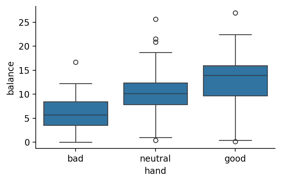
That there’s a linear trend such that balance increases going from bad -> neutral -> good
How do we test this hypothesis? We can just create a new variable that treats our category levels as if they were a continuous variable!
This only makes sense, if there is some natural ordering to the category levels because it assumes that the increment from bad -> neutral is the same as from neutral -> good. In our case this is defensible, as moving from left-to-right on the x-axis above is akin to moving along a continuous variable anchored by bad and good end-points. But this wouldn’t make a lot of sense of our levels didn’t have a natural ordering (e.g. dog, human, bird)
Concretely we’re trying to estimate the slope of a line that connects bad -> good
We can use a little linear algebra to see what this means:
bad = df.filter(col('hand') == 'bad')['balance'].mean()
good = df.filter(col('hand') == 'good')['balance'].mean()
neutral = df.filter(col('hand') == 'neutral')['balance'].mean()

# Put the means of each hand level in an array ordered in the way we want
means = np.array([bad, neutral, good])

numerical_hand = np.array([-1, 0, 1])

np.dot(means, numerical_hand)
np.float64(7.084900000000006)
This captures the equivalent of a slope that reflect: “change in balance” for 1-unit change in hand!
Let’s try to estimate this using a regression following this procedure:
Create a new variable that replaces levels of a categorical variable continuous values
To support unbalanced data and intepretabiltiy - make sure the continuous values are centered at zero (just like a true continuous variable)
(Optional) Use fractional numerical values that add up to one to interpret the regression slope as a 1-unit change in the categorical variable
Run a new regression using the variable you just created with no categorical coding
Let’s do that now:
# We can use the .replace() method to convert values of one column to new values
df = df.with_columns(
    hand_slope = col('hand').replace({'bad': -1, 'neutral': 0, 'good': 1}).cast(float)
)
df.head()
| skill | hand | limit | balance | hand_slope |
|---|---|---|---|---|
| str | str | str | f64 | f64 |
| "expert" | "bad" | "fixed" | 4.0 | -1.0 |
| "expert" | "bad" | "fixed" | 5.55 | -1.0 |
| "expert" | "bad" | "fixed" | 9.45 | -1.0 |
| "expert" | "bad" | "fixed" | 7.19 | -1.0 |
| "expert" | "bad" | "fixed" | 5.71 | -1.0 |
oneway_continuous = ols('balance ~ hand_slope', data=df.to_pandas()).fit()
print(oneway_continuous.summary(slim=True))
                            OLS Regression Results
==============================================================================
Dep. Variable:                balance   R-squared:                       0.331
Model:                            OLS   Adj. R-squared:                  0.329
No. Observations:                 300   F-statistic:                     147.5
Covariance Type:            nonrobust   Prob (F-statistic):           7.58e-28
==============================================================================
                 coef    std err          t      P>|t|      [0.025      0.975]
------------------------------------------------------------------------------
Intercept      9.7715      0.238     41.032      0.000       9.303      10.240
hand_slope     3.5424      0.292     12.145      0.000       2.968       4.116
==============================================================================

Notes:
[1] Standard Errors assume that the covariance matrix of the errors is correctly specified.
In the output above the intercept is the grand-mean. Why? Because out continuous variable is centered!
Wait, but out hand_slope doesn’t look the value we calculated above…what’s going on?
It turns out converting our categorical levels using -1, 0, 1, the regression slope is twice as long as we would expect if our categorical variable was a true continuous variable. So our our estimate slope is half as big as it should be.
oneway_continuous.params['hand_slope'] * 2
np.float64(7.084899999999991)
This does not affect the t-statistic and p-values of our parameter - just the estimate itself.
To make things more interpretable the fix is easy - following step 3 above and using fractional values who’s absolute value adds up to 1
Let’s see this in code and visually:
# Original approach
continuous_hand = np.array([-1, 0, 1])

# Slope = max - min
np.max(continuous_hand) - np.min(continuous_hand)
np.int64(2)
# If we have to divide our estimate by 2, we can just divide the continous values by 2 instead!
lincon = continuous_hand / 2

# This is actually what we want for interpretation
lincon
array([-0.5, 0. , 0.5])
# Slope is now 1 not 2
# Slope = max - min
np.max(lincon) - np.min(lincon)
np.float64(1.0)
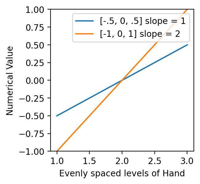
And visually we can see over the same range of x-values (continuous version of hand levels), [-1, 0, 1], have a slope of 2 and thus produce a coefficient that’s half as big as the value we would like
plt.figure(figsize=(3,3))
plt.plot([1,2,3], lincon, label='[-.5, 0, .5] slope = 1')
plt.plot([1,2,3], continuous_hand, label='[-1, 0, 1] slope = 2')
plt.ylim([-1, 1]);
plt.xlabel('Evenly spaced levels of Hand');
plt.ylabel('Numerical Value')
plt.legend();
Challenge (mini)#
Using the example and explanation above, create/replace the column we created (continuous version of hand) to use values that have a slope of 1.
Then use that new column to run a univariate regression. What does the parameter estimate look like now?
# Your code here
# Solution
df = df.with_columns(
    hand_slope = col('hand').replace({'bad': -.5, 'neutral': 0, 'good': .5}).cast(float)
)
df.head()
| skill | hand | limit | balance | hand_slope |
|---|---|---|---|---|
| str | str | str | f64 | f64 |
| "expert" | "bad" | "fixed" | 4.0 | -0.5 |
| "expert" | "bad" | "fixed" | 5.55 | -0.5 |
| "expert" | "bad" | "fixed" | 9.45 | -0.5 |
| "expert" | "bad" | "fixed" | 7.19 | -0.5 |
| "expert" | "bad" | "fixed" | 5.71 | -0.5 |
# Solution
oneway_continuous = ols('balance ~ hand_slope', data=df.to_pandas()).fit()
print(oneway_continuous.summary(slim=True))
                            OLS Regression Results
==============================================================================
Dep. Variable:                balance   R-squared:                       0.331
Model:                            OLS   Adj. R-squared:                  0.329
No. Observations:                 300   F-statistic:                     147.5
Covariance Type:            nonrobust   Prob (F-statistic):           7.58e-28
==============================================================================
                 coef    std err          t      P>|t|      [0.025      0.975]
------------------------------------------------------------------------------
Intercept      9.7715      0.238     41.032      0.000       9.303      10.240
hand_slope     7.0849      0.583     12.145      0.000       5.937       8.233
==============================================================================

Notes:
[1] Standard Errors assume that the covariance matrix of the errors is correctly specified.
Comparison to Polynomial Coding#
It turns out that this is what polynomial coding is doing when we use C(hand, Poly)! Technically, it estimates all possible polynomials (linear, quadratic, cubic, etc.), but let’s just focus on the linear one to build our intuition:
poly_model = ols('balance ~ C(hand, Poly)', data=df.to_pandas())
poly_fit = poly_model.fit()

poly_fit.params
Intercept                  9.771500
C(hand, Poly).Linear       3.114876
C(hand, Poly).Quadratic   -3.986422
dtype: float64
We’re going to manually create the polynomial contrasts like ols does for us and then use the same approach as earlier to replace our categorical variable with a new continuous one:
from patsy.contrasts import Poly

# Levels in the order they appear by default in the model
levels = ['bad', 'good','neutral']

# Generate a matrix using our predictor variables
# These are the comparisons our parameters above reflect!
poly_codes = Poly().code_without_intercept(levels)


poly_codes.column_suffixes
poly_codes.matrix
['.Linear', '.Quadratic']
array([[-7.07106781e-01,  4.08248290e-01],
       [-1.69402794e-17, -8.16496581e-01],
       [ 7.07106781e-01,  4.08248290e-01]])
Let’s just grab the linear one:
poly_lincon = poly_codes.matrix[:,0]
And then replace our factor levels with it:
df = df.with_columns(
    hand_poly_Linear = col('hand').replace({
        'bad': poly_lincon[0],
        'good': poly_lincon[1],
        'neutral': poly_lincon[2]
    }).cast(float)
)

ols('balance ~ hand_poly_Linear', data=df.to_pandas()).fit().params
Intercept           9.771500
hand_poly_Linear    3.114876
dtype: float64
And we can see that our “continu-fied” version of hand, using the same continuous values that Poly used, produces the same (linear) parameter estimate!
poly_fit.params
Intercept                  9.771500
C(hand, Poly).Linear       3.114876
C(hand, Poly).Quadratic   -3.986422
dtype: float64
Wrap-up Challenge#
1.#
Your colleage has estimated the following model and is very excited about the significant result on the parameter estimate skill_con below. Leveraging what you’ve learned about continuous and categorical predictors, help them understand it by answering the following questions:
What does the parameter estimate represent?
How does it affect the interpretation of the
hand_lincon:skill_coninteraction estimate?Does this estimate test the difference they intended to test? Why or why not?
Use any coding/visualization approach you would like to support your answers
Your response here
# Your colleague's code - you can just run this cell
df = df.with_columns(
    hand_lincon = col('hand').replace({
        'bad': 1,
        'neutral': 2,
        'good': 3
    }).cast(float),
    skill_con = col('skill').replace({
        'average': .5,
        'expert': -.5
    }).cast(float)
)

model_h = ols('balance ~ hand_lincon * skill_con', data=df.to_pandas()).fit()
print(model_h.summary(slim=True))
                            OLS Regression Results
==============================================================================
Dep. Variable:                balance   R-squared:                       0.366
Model:                            OLS   Adj. R-squared:                  0.360
No. Observations:                 300   F-statistic:                     56.99
Covariance Type:            nonrobust   Prob (F-statistic):           4.17e-29
=========================================================================================
                            coef    std err          t      P>|t|      [0.025      0.975]
-----------------------------------------------------------------------------------------
Intercept                 2.6866      0.615      4.365      0.000       1.475       3.898
hand_lincon               3.5424      0.285     12.434      0.000       2.982       4.103
skill_con                -4.9765      1.231     -4.043      0.000      -7.399      -2.554
hand_lincon:skill_con     2.1261      0.570      3.731      0.000       1.005       3.247
=========================================================================================

Notes:
[1] Standard Errors assume that the covariance matrix of the errors is correctly specified.
# Your code here
# Solution
# It represents the slope of skill when hand_lincon is 0

# Get predictions when hand_lincon is 0 to verify
hand_lincon = np.repeat(0, df.height)
skill_con = df['skill_con'].to_numpy()
preds = model_h.predict({'hand_lincon': hand_lincon, 'skill_con': skill_con})

# Fit model and grab skill_con coefficient
ols('preds ~ skill_con', data=pl.DataFrame({'preds': preds, 'skill_con': skill_con})).fit().params['skill_con']
np.float64(-4.976533333333325)
2.#
Fix your colleague’s work by estimating a new multiple regression using continous versions of skill, hand, and their interaction. Create your new variables to test:
a linear contrast of
hand, such that balance increases frombad->neutral->gooda linear contrast of
skillsuch that balance increases fromaverage->expert
Verify that your parameter estimate reflect the hypothesis you expect by using the means of each factor level like we’ve demonstrated in this notebook
How do these estimates compare to the ones your colleage got above?
# Your code here
# Solution
df = df.with_columns(
    hand_lincon = col('hand').replace({
        'bad': -.5,
        'neutral': 0,
        'good': .5
    }).cast(float),
    skill_con = col('skill').replace({
        'average': .5,
        'expert': -.5
    }).cast(float)
)

model_h = ols('balance ~ hand_lincon * skill_con', data=df.to_pandas()).fit()
print(model_h.summary(slim=True))
                            OLS Regression Results
==============================================================================
Dep. Variable:                balance   R-squared:                       0.366
Model:                            OLS   Adj. R-squared:                  0.360
No. Observations:                 300   F-statistic:                     56.99
Covariance Type:            nonrobust   Prob (F-statistic):           4.17e-29
=========================================================================================
                            coef    std err          t      P>|t|      [0.025      0.975]
-----------------------------------------------------------------------------------------
Intercept                 9.7715      0.233     42.008      0.000       9.314      10.229
hand_lincon               7.0849      0.570     12.434      0.000       5.964       8.206
skill_con                -0.7243      0.465     -1.557      0.121      -1.640       0.191
hand_lincon:skill_con     4.2522      1.140      3.731      0.000       2.010       6.495
=========================================================================================

Notes:
[1] Standard Errors assume that the covariance matrix of the errors is correctly specified.
# Solution
expert = df.filter(col('skill') == 'expert')['balance'].mean()
average = df.filter(col('skill') == 'average')['balance'].mean()

bad = df.filter(col('hand') == 'bad')['balance'].mean()
neutral = df.filter(col('hand') == 'neutral')['balance'].mean()
good = df.filter(col('hand') == 'good')['balance'].mean()
# skill_con is the same as expert - average

# The dot product calculates this:
# -1 * expert + 1 * average
np.dot([expert, average], [-1, 1])
np.float64(-0.7243333333333322)
# hand_lincon is the linear trend from bad -> neutral -> good

# The dot product calculates this:
# -1 * bad + 0 * netural + 1 * good
np.dot([bad, neutral, good], [-1, 0, 1])
np.float64(7.084899999999999)
We can think about the interaction as difference-of-differences in 2 ways:
The difference between
skilldifferences at each level ofhand
average_hands = cell_means.filter(col('skill') == 'average')
average_hands
| hand | skill | balance |
|---|---|---|
| str | str | f64 |
| "bad" | "average" | 4.5866 |
| "good" | "average" | 13.7976 |
| "neutral" | "average" | 9.8438 |
expert_hands = cell_means.filter(col('skill') == 'expert')
expert_hands
| hand | skill | balance |
|---|---|---|
| str | str | f64 |
| "bad" | "expert" | 7.2964 |
| "good" | "expert" | 12.2552 |
| "neutral" | "expert" | 10.8494 |
hands_diffs = (average_hands['balance'] - expert_hands['balance']).to_numpy()

# Rearrange the hand levels into [bad, neutral, good] order
hands_diffs = np.array([hands_diffs[0], hands_diffs[2], hands_diffs[1]])

# Linear contrast across differences
np.dot(hands_diffs, [-1, 0, 1])
np.float64(4.252199999999996)
The difference between
handdifferences at each level ofskill
# Below we create [expert, average] array for each hand level
bad_skill = cell_means.filter(col('hand') == 'bad').sort(by='skill', descending=True)['balance'].to_numpy()

neutral_skill = cell_means.filter(col('hand') == 'neutral').sort(by='skill', descending=True)['balance'].to_numpy()

good_skill = cell_means.filter(col('hand') == 'good').sort(by='skill', descending=True)['balance'].to_numpy()
# E.g.
bad_skill
array([7.2964, 4.5866])
# Stack into 2 (skill) x 3 (hand) arrray
# in the order of hand levels we want to test
skills = np.column_stack([bad_skill, neutral_skill, good_skill])
skills
array([[ 7.2964, 10.8494, 12.2552],
       [ 4.5866,  9.8438, 13.7976]])
# Calculate the linear contrast
lin_con = np.dot(skills, [-1, 0, 1])
lin_con
array([4.9588, 9.211 ])
# And the difference between those
lin_con[1] - lin_con[0]
np.float64(4.252199999999995)