Models V: Categorical Predictors (2-levels)

Models V: Categorical Predictors (2-levels)#

So far we’ve been using ols to perform univariate and multiple regression with continuous predictor variables. But often you’ll also be working with categorical predictor variables. In this notebook we’ll discuss how to build models using:

a categorical variable with 2 levels
a categorical variable with 2 levels + a continuous variable
a categorical variable with 2 levels, a continuous variable, and an interaction term

Slides for reference#

Modeling Data V (slides)

Data#

Let’s return to the credit card dataset we used in Notebook 02_models

This is a smaller version of that dataset with observations from 76 different people with the following columns:

Variable	Description
Income	in thousand dollars
Limit	credit limit
Rating	credit rating
Cards	number of credit cards
Age	in years
Education	years of education
Gender	male or female
Student	student or not
Married	married or not
Ethnicity	African American, Asian, Caucasian
Balance	average credit card debt

import numpy as np
import polars as pl
from polars import col
import seaborn as sns
import matplotlib.pyplot as plt
from statsmodels.formula.api import ols
from statsmodels.stats.anova import anova_lm

# Load data
df = pl.read_csv('./data/credit-mini.csv')
df

shape: (76, 11)

Income	Limit	Rating	Cards	Age	Education	Gender	Student	Married	Ethnicity	Balance
f64	i64	i64	i64	i64	i64	str	str	str	str	i64
20.918	1233	128	3	47	18	"Female"	"Yes"	"Yes"	"Asian"	16
10.842	4391	358	5	37	10	"Female"	"Yes"	"Yes"	"Caucasian"	1216
29.705	3351	262	5	71	14	"Female"	"No"	"Yes"	"Asian"	148
76.348	4697	344	4	60	18	"Male"	"No"	"No"	"Asian"	108
30.622	3293	251	1	68	16	"Male"	"Yes"	"No"	"Caucasian"	532
…	…	…	…	…	…	…	…	…	…	…
107.841	10384	728	3	87	7	"Male"	"No"	"No"	"African American"	1597
27.47	2820	219	1	32	11	"Female"	"No"	"Yes"	"Asian"	0
15.741	4788	360	1	39	14	"Male"	"No"	"Yes"	"Asian"	689
16.751	4706	353	6	48	14	"Male"	"Yes"	"No"	"Asian"	1255
14.084	855	120	5	46	17	"Female"	"No"	"Yes"	"African American"	0

Categorical Predictor w/ 2 levels#

Let’s use ols to explore the example discussed in class in more detail: do students have a different balance than non-students?

We’ll fit 2 models:

a compact model that only includes the intercept
an augmented model that includes a categorical predictor for Student which has 2 levels (Yes and No)

We can tell ols to treat a variable as categorical by wrapping it in C()

Then we’ll test whether it’s worth it to add Student as a predictor to the model by comparing them like we have before:

# Compact Model
c_model = ols('Balance ~ 1', data=df.to_pandas())
c_results = c_model.fit()

# Augmented Model
# Treat "Student" as a categorical variable
a_model = ols('Balance ~ C(Student)', data=df.to_pandas())
a_results = a_model.fit()

# Compare models - worth it?
anova_lm(c_results, a_results)

	df_resid	ssr	df_diff	ss_diff	F	Pr(>F)
0	75.0	2.028075e+07	0.0	NaN	NaN	NaN
1	74.0	1.721872e+07	1.0	3.062040e+06	13.159573	0.000523

It’s worth it!

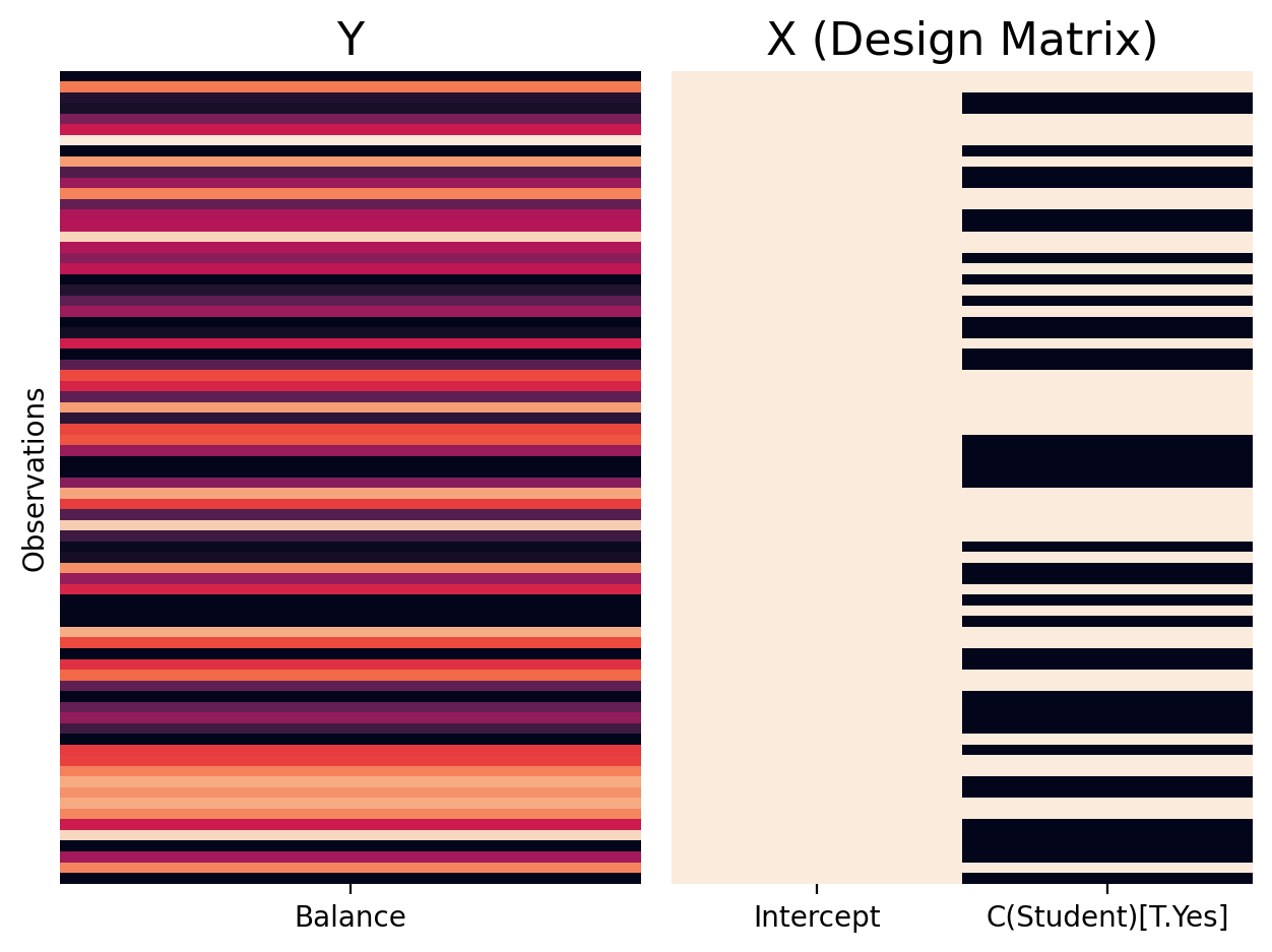
Let’s inspect our augmented model’s design matrix to try to understand how ols is representing our categorical variable Student

# First 6 rows
a_model.exog[:5, :]

array([[1., 1.],
       [1., 1.],
       [1., 0.],
       [1., 0.],
       [1., 1.]])

If we look at our DataFrame, we can see that by default C() has converted: No = 0 and Yes = 1

df.select('Balance', 'Student').head()

shape: (5, 2)

Balance	Student
i64	str
16	"Yes"
1216	"Yes"
148	"No"
108	"No"
532	"Yes"

Sometimes it’s helpful to see the entire design matrix, especially as we move onto categorical variables with more than 2 levels in future notebooks.

We’ve provided a helper function you can use that takes a model as input. You can see each observation plotted alongside how we’ve encoded Student in the design matrix (beige = 1; black = 0):

from helpers import plot_design_matrix

plot_design_matrix(a_model)

../../_images/2e5bc837681b236af31d7b811bebb92eff1e5a3d6908268f53f70d6f72a1ebb3.png

Let’s inspect the .summary() to look at the parameter estimates for the model Intercept and C(Student)[T.Yes]

What do the intercept $\hat{\beta}_0$ and slope $\hat{\beta}_1$ here represent?

To answer this question we need to understand what it means to think about levels of a category in terms of the slopes of lines that we can estimate. And how the 0s and 1s in the design matrix relate to this…

# slim=True just removes some extra information we don't currently need to save space
print(a_results.summary(slim=True)) 

                            OLS Regression Results                            
==============================================================================
Dep. Variable:                Balance   R-squared:                       0.151
Model:                            OLS   Adj. R-squared:                  0.140
No. Observations:                  76   F-statistic:                     13.16
Covariance Type:            nonrobust   Prob (F-statistic):           0.000523
=====================================================================================
                        coef    std err          t      P>|t|      [0.025      0.975]
-------------------------------------------------------------------------------------
Intercept           463.2368     78.252      5.920      0.000     307.317     619.156
C(Student)[T.Yes]   401.4474    110.664      3.628      0.001     180.944     621.951
=====================================================================================

Notes:
[1] Standard Errors assume that the covariance matrix of the errors is correctly specified.

Introduction to Categorical Coding Schemes#

Let’s think about about what it means to calculate a slope between 2 levels of a categorical variable.

We typically define the slope as the “change in y for 1-unit change in x” - this makes sense when both variables are continuous - e.g. how much a person’s Balance (y) increases for every additional year they’re alive Age (x).

But what is a “unit change in x” if x is a categorical variable like Student?

Its the difference between going from the mean of first level No to the mean of the second level Yes!

The mean difference is the regression slope $\hat{\beta_1}$

Treatment (Dummy) Coding#

While there are actually many ways to encode a categorical variable as columns of our design matrix, this intuitive idea is the default in both Python and R and is called treatment (dummy) coding.

It uses the intercept to estimate the mean of one of the levels of your categorical variable as a reference level, and encodes the other levels as mean differences from that reference level.

In the case of a variable with just 2 levels - this is just the mean difference between both levels, i.e. between Student=No and Student=Yes

# Get mean balance for each level separately
student_yes = df.filter(col('Student')=='Yes').select('Balance').mean()[0,0]
student_no = df.filter(col('Student')=='No').select('Balance').mean()[0,0]

print(f'Student: Yes = {student_yes:.3f}, No = {student_no:.3f}')
print(f"Mean Difference (Yes - No) = {student_yes - student_no:.5f}")

Student: Yes = 864.684, No = 463.237
Mean Difference (Yes - No) = 401.44737

# beta 0 = mean of No
# beta 1 = mean difference
a_results.params

Intercept            463.236842
C(Student)[T.Yes]    401.447368
dtype: float64

To make this more concrete, let’s add a new column to our DataFrame called Student_Dummy that represents Student just like our design matrix does:

Challenge#

Use when and lit that we’ve imported for you below to create a new column in df called Student_Dummy that encodes Yes = 1 and No = 0 for the Student variable.

Hint: You can use .alias() at the end of your when statement to give your new column a name.

from polars import when, lit

# Solution
df = df.with_columns(
    when(col('Student') == 'Yes')
    .then(lit(1))
    .otherwise(lit(0))
    .alias('Student_Dummy')
)

df.head()

shape: (5, 12)

Income	Limit	Rating	Cards	Age	Education	Gender	Student	Married	Ethnicity	Balance	Student_Dummy
f64	i64	i64	i64	i64	i64	str	str	str	str	i64	i32
20.918	1233	128	3	47	18	"Female"	"Yes"	"Yes"	"Asian"	16	1
10.842	4391	358	5	37	10	"Female"	"Yes"	"Yes"	"Caucasian"	1216	1
29.705	3351	262	5	71	14	"Female"	"No"	"Yes"	"Asian"	148	0
76.348	4697	344	4	60	18	"Male"	"No"	"No"	"Asian"	108	0
30.622	3293	251	1	68	16	"Male"	"Yes"	"No"	"Caucasian"	532	1

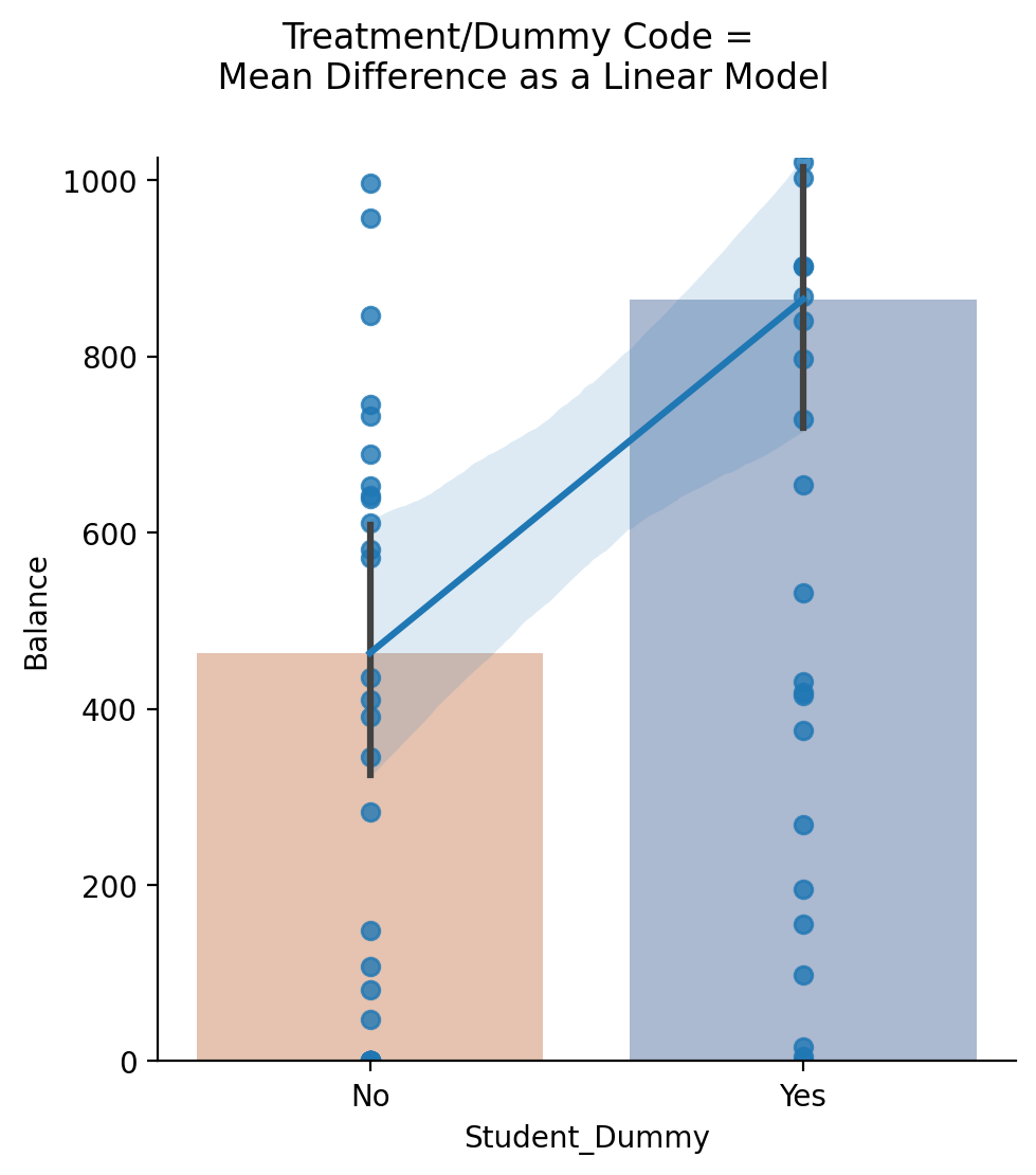
Let’s use the new column you made to create a figure and build our intuitions visually.
First, we’ll use sns.barplot to show the mean Balance of each level of Student
Then, we’ll ask sns.regplot to estimate and plot a regression line between our Student_Dummy and Balance variables; seaborn uses ols behind-the-scenes to do this!

You’ll see below that the slope of sns.regplot going from 0 to 1 is the same as the difference between bars

x_order = ['No', 'Yes']

# Create grid
grid = sns.FacetGrid(data=df.to_pandas(),height=5) ;

# Add a barpplot; we use map_dataframe so we can control hue separately for this layer
grid.map_dataframe(sns.barplot, 'Student', 'Balance', hue='Student',palette='deep', order=x_order, alpha=.5);

# Add a regression using our new column
grid.map_dataframe(sns.regplot, 'Student_Dummy', 'Balance')

# Aesthetics
grid.set(ylim=(0,1025));
grid.figure.suptitle("Treatment/Dummy Code =\n Mean Difference as a Linear Model", y=1.1);

../../_images/eb9f2f0284c570087939878dc96213fa6df760aee3a6515e8f28b070553fc6cb.png

We can also see this by estimating a new model using our newly created column Student_Dummy as a predictor and comparing its output to our original augmented model:

dummy_model = ols('Balance ~ Student_Dummy', data=df.to_pandas())
dummy_results = dummy_model.fit()

dummy_results.params

Intercept        463.236842
Student_Dummy    401.447368
dtype: float64

a_results.params

Intercept            463.236842
C(Student)[T.Yes]    401.447368
dtype: float64

Interpreting parameter estimates#

In our model our parameters represent:

$\hat{\beta_0} = StudentNo_{mean}$ (reference level)
$\hat{\beta_1} = StudentYes_{mean} - StudentNo_{mean}$

By default ols will use alphabetically sort the levels of your categorical predictor and use the first one as the reference level. In our case this is No as as N comes before Y alphabetically.

But we can be more explicit and even control what group is the reference category. Let’s switch it to Student = Yes

We can do this by passing a second argument to C() in addition to our column name. We can use Treatment(reference='category_level') to tell ols that the reference category is Yes

# Set the reference group (intercept) to 'Yes'
ref_yes = ols("Balance ~ C(Student, Treatment(reference='Yes'))", data=df.to_pandas())

print(ref_yes.fit().summary(slim=True)) 

                            OLS Regression Results                            
==============================================================================
Dep. Variable:                Balance   R-squared:                       0.151
Model:                            OLS   Adj. R-squared:                  0.140
No. Observations:                  76   F-statistic:                     13.16
Covariance Type:            nonrobust   Prob (F-statistic):           0.000523
================================================================================================================
                                                   coef    std err          t      P>|t|      [0.025      0.975]
----------------------------------------------------------------------------------------------------------------
Intercept                                      864.6842     78.252     11.050      0.000     708.765    1020.604
C(Student, Treatment(reference='Yes'))[T.No]  -401.4474    110.664     -3.628      0.001    -621.951    -180.944
================================================================================================================

Notes:
[1] Standard Errors assume that the covariance matrix of the errors is correctly specified.

Now the intercept is the mean of Student = Yes and the slope is No - Yes

student_yes

864.6842105263158

student_no - student_yes

-401.44736842105266

Inspecting the design matrix we can see that the coding has simply been flipped from our augmented model above:

# No = 1
# Yes = 0
ref_yes.exog[:5, :]

array([[1., 0.],
       [1., 0.],
       [1., 1.],
       [1., 1.],
       [1., 0.]])

# Originally we had
# No = 0
# Yes = 1
a_model.exog[:5, :]

array([[1., 1.],
       [1., 1.],
       [1., 0.],
       [1., 0.],
       [1., 1.]])

And just to confirm, we can see that the t-statistic and p-value that ols gives us is that same as running an independent t-test using scipy:

from scipy.stats import ttest_ind

results = ttest_ind(
    df.filter(col('Student') == 'No').select('Balance').to_numpy(),
    df.filter(col('Student') == 'Yes').select('Balance').to_numpy())

print(f"Independent samples t-test t({results.df[0]}) = {results.statistic[0]:.3f}, p = {results.pvalue[0]:.5f}")

Independent samples t-test t(74.0) = -3.628, p = 0.00052

Or in APA style:

print(f"Independent samples t-test t({results.df[0]}) = {results.statistic[0]:.3f}, p < .001")

Independent samples t-test t(74.0) = -3.628, p < .001

Categorical (2-level) and Continuous Predictors#

In the previous notebook 02_models we saw that Income was also a meaningful predictor of Balance:

grid = sns.lmplot(data=df, x='Income', y='Balance')

Let’s expand our model to account for this relationship when looking at the difference between Students and non-Students.

Specifically let’s estimate a multiple regression that asks: do students have difference Balances than non-students when accounting for Income?

\[ \hat{Balance}_{i}= \beta_0 + \beta_1 Student + \beta_2 Income \]

We’ll also estimate another univariate regression that only looks at the relationship between Balance and Income:

\[ \hat{Balance}_{i}= \beta_0 + \beta_1 Income \]

Challenge#

Estimate the two models above
Use anova_lm to compare both models. Is the multiple regression worth it?
Use anova_lm to compare the multiple regression to a_results, your original augmented model (univariate with only Student as a predictor). Is the multiple regression worth it?
Create a new dataframe called df_models that includes the following columns:

Balance the original balance variable
Student the original student variable
Income the original income variable
balance_pred_si the .fittedvalues attribute of the multiple regression
resid_si the .resid attribute of the multiple regression
balance_pred_i the .fittedvalues attribute of the univariate regression
resid_i the .resid attribute of the univariate regression
balance_pred_s the .fittedvalues from the univariate a_results we estimated above
resid_s the .resid from the univariate a_results we estimated above

# Solution
# Student only
s_model = ols('Balance ~ C(Student)', data=df.to_pandas())
s_results = s_model.fit()

# Income only
i_model = ols('Balance ~ Income', data=df.to_pandas())
i_results = i_model.fit()

# Student + Income
si_model = ols('Balance ~ C(Student) + Income', data=df.to_pandas())
si_results = si_model.fit()

# S+I vs S
anova_lm(s_results, si_results)

	df_resid	ssr	df_diff	ss_diff	F	Pr(>F)
0	74.0	1.721872e+07	0.0	NaN	NaN	NaN
1	73.0	1.374135e+07	1.0	3.477369e+06	18.473293	0.000052

# S+I vs I
anova_lm(i_results, si_results)

	df_resid	ssr	df_diff	ss_diff	F	Pr(>F)
0	74.0	1.685200e+07	0.0	NaN	NaN	NaN
1	73.0	1.374135e+07	1.0	3.110658e+06	16.525165	0.00012

# Solution
df_models = df.select(
    col('Balance'),
    col('Student'),
    col('Income'),
    balance_pred_si = si_results.fittedvalues.to_numpy(),
    resid_si = si_results.resid.to_numpy(),
    balance_pred_i = i_results.fittedvalues.to_numpy(),
    resid_i = i_results.resid.to_numpy(),
    balance_pred_s = a_results.fittedvalues.to_numpy(),
    resid_s = a_results.resid.to_numpy(),
)
df_models.head()

shape: (5, 9)

Balance	Student	Income	balance_pred_si	resid_si	balance_pred_i	resid_i	balance_pred_s	resid_s
i64	str	f64	f64	f64	f64	f64	f64	f64
16	"Yes"	20.918	727.826282	-711.826282	526.484832	-510.484832	864.684211	-848.684211
1216	"Yes"	10.842	672.269098	543.730902	471.318923	744.681077	864.684211	351.315789
148	"No"	29.705	371.643114	-223.643114	574.593491	-426.593491	463.236842	-315.236842
108	"No"	76.348	628.823915	-520.823915	829.963033	-721.963033	463.236842	-355.236842
532	"Yes"	30.622	781.332328	-249.332328	579.614049	-47.614049	864.684211	-332.684211

Interpreting Parameter Estimates#

Now that we know the multiple regression is worth it, let’s interpret the parameter estimates.

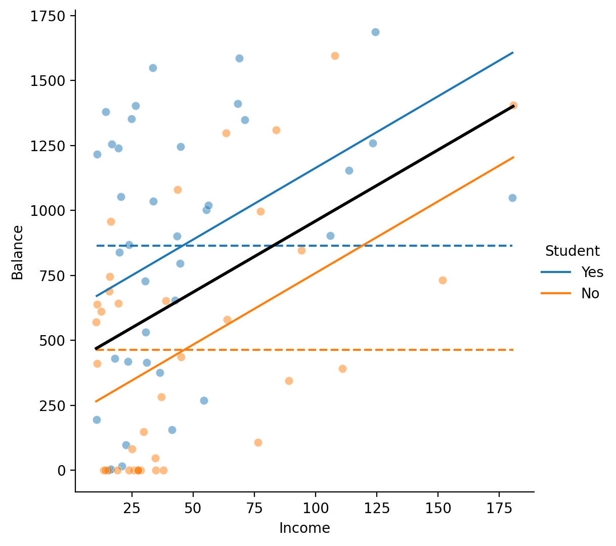
Let’s build some visual intuitions by plotting the predictions from the multiple regression and each separate univariate regression to see what’s changing. In the figure below:

The scatterplot points represent the raw data separated by the levels of Student
In solid black line is the relationshion between Income and Balance if we ignore Student
The dashed colored lines represent the relationship between Balance and Student if we ignore Income
The solid colored lines represent the relationship between Balance and Income if we account for difference in the intercepts for each level of Student

# Create grid
grid = sns.FacetGrid(data=df_models.to_pandas(), hue="Student", height=5.5, aspect=1);

# Plot data
grid.map(sns.scatterplot, "Income", "Balance",alpha=.5);

# Plot our predictions from student only model
grid.map(sns.lineplot, "Income", "balance_pred_s", ls='--');

# Plot our predictions from income only model
grid.map(sns.lineplot, "Income", "balance_pred_i", ls='-', color='black', lw=2);

# Plot our predictions student + income
grid.map(sns.lineplot, "Income", "balance_pred_si");

# Aesthetics
grid.set(ylabel='Balance');
grid.add_legend();

../../_images/ccd94147e6fc0975cee85672cfbb1d483b35a00f33926633f005bac87fc50b48.png

Let’s take a look at the parameter estimates…

si_results.params

Intercept            207.855285
C(Student)[T.Yes]    404.633047
Income                 5.513813
dtype: float64

$\hat{\beta_0}$ is supposed to be the mean of Student = No…but its not

$\hat{\beta_1}$ is supposed to be the mean difference between Student = Yes and Student = No…but its not

$\hat{\beta_2}$ is supposed to be the slope of Income…but it doesn’t match our univariate regression i_results

Our model with just Student shows that the $\hat{\beta}_0$ was the mean of Student = No

a_results.params

Intercept            463.236842
C(Student)[T.Yes]    401.447368
dtype: float64

And our model with just Income shows that the $\hat{\beta}_1$ was the slope of Income

i_results.params

Intercept    411.959178
Income         5.474981
dtype: float64

What’s going on?

Remember what we learned in notebooks 02_models and 03_models:

In the GLM, we interpret each parameter estimate assuming other parameter estimates = 0

Because of this:

$\hat{\beta_0}$ is the mean of Student = No when Income = 0

$\hat{\beta_1}$ is the mean difference between Student = Yes and Student = No when Income = 0

$\hat{\beta_2}$ is the slope of Income when Student = 0 (No)

Challenge#

Can you make the parameter estimates more interpretable using an approach we learned in class and demonstrated in 02_models? Think about how to change what value the regression “fixes” Income to from 0 to something more useful…

Fit a new more interpretable multiple regression called si_interp_model using Student and Income as predictors and save the results to si_interp_results
Compare your parameter estimates from .summary() or .params to the estimates from the original multiple regression. What do you notice?

# Solution
si_interp_model = ols('Balance ~ C(Student) + center(Income)', data=df.to_pandas())

si_interp_results = si_interp_model.fit()

print(si_interp_results.summary(slim=True))

                            OLS Regression Results                            
==============================================================================
Dep. Variable:                Balance   R-squared:                       0.322
Model:                            OLS   Adj. R-squared:                  0.304
No. Observations:                  76   F-statistic:                     17.37
Covariance Type:            nonrobust   Prob (F-statistic):           6.75e-07
=====================================================================================
                        coef    std err          t      P>|t|      [0.025      0.975]
-------------------------------------------------------------------------------------
Intercept           461.6440     70.383      6.559      0.000     321.371     601.917
C(Student)[T.Yes]   404.6330     99.538      4.065      0.000     206.254     603.012
center(Income)        5.5138      1.283      4.298      0.000       2.957       8.071
=====================================================================================

Notes:
[1] Standard Errors assume that the covariance matrix of the errors is correctly specified.

Visualizing intutions#

Hopefully you remembered that you can center a predictor to change what the fixed value is when intepreting other parameters. It doesn’t change the estimate for what you’re centering (Income), but it always changes the intercept and other categorical parameters!

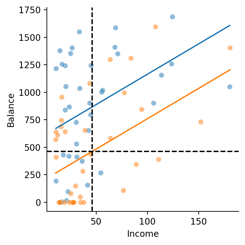
Let’s visualize the effect of centering a predictor - we’ll annotate the same plot as earlier illustrating the shift in coefficient interpretation:

We’ll add a vertical line for Income = mean(Income) and a horizontal line for the mean of Student = No- this is our model intercept
The vertical distance between this point and where it intersect the blue line is $\beta_1$ - mean difference between Yes and No when Income is at its mean

# Create grid
grid = sns.FacetGrid(data=df_models.to_pandas(), hue="Student", height=4)

# Plot data
grid.map(sns.scatterplot, "Income", "Balance",alpha=.5)

# Plot our predictions student + income
grid.map(sns.lineplot, "Income", "balance_pred_si")

# Plot Income mean
grid.map(plt.axvline, x=df_models['Income'].mean(), color="black", ls='--');

# Plot mean for Student = 0
grid.map(plt.axhline, y=student_no, color="black", ls='--');

# Aesthetics
grid.set(ylabel='Balance');

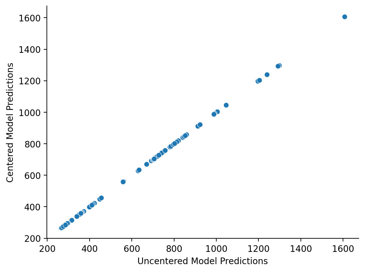
../../_images/bcb07865a3c47720edf25185d6868dfe6b74621ec9d30290154bce0ee7cced5f.png

You’ll also notice that centering does not change model predictions. It only changes how we interpret the parameter estimates from our model

ax = sns.scatterplot(
    x=si_results.fittedvalues, # predictions fro un-centered model
    y=si_interp_results.fittedvalues, # predictions for centered model
)
ax.set(xlabel='Uncentered Model Predictions', ylabel='Centered Model Predictions');
sns.despine();

../../_images/c91e617a733f93f41934050c7aaf318132067d0ed7b392d91d8e27cce7d688ad.png

In notebook 03_models we learned that we can use .predict() to generate predictions from our model by fixing one or more of our predictors at certain values.

Let’s do that now to get our predicted estimates of the average Balance for each level of Student when Income is fixed at it’s mean of 46.03 - this is what our parameter estimate for Student is

# Create 1-row dataframes to pass into .predict()
student_no_x =pl.DataFrame({
    'Income': df['Income'].mean(),
    'Student': 'No'
})

student_yes_x =pl.DataFrame({
    'Income': df['Income'].mean(),
    'Student': 'Yes'
})

# Generate predictions
student_no_prediction = si_interp_results.predict(student_no_x.to_pandas())

student_yes_prediction = si_interp_results.predict(student_yes_x.to_pandas())

print(f"Student (No): {student_no:.3f}")
print(f"Student (Yes): {student_yes:.3f}")

print(f"Student (No prediction): {student_no_prediction[0]:.3f}")
print(f"Student (Yes prediction): {student_yes_prediction[0]:.3f}")

print(f"Student (Yes prediction - No prediction): {student_yes_prediction[0] - student_no_prediction[0]:.3f}")

Student (No): 463.237
Student (Yes): 864.684
Student (No prediction): 461.644
Student (Yes prediction): 866.277
Student (Yes prediction - No prediction): 404.633

And we can verify that:

$\beta_0$ = $\hat{balance}_{\text{student\_no}}$ when $Income = Income_{mean}$
$\beta_1$ = $\hat{balance}_{\text{student\_yes}}$ - $\hat{balance}_{\text{student\_no}}$ when $Income = Income_{mean}$

si_interp_results.params

Intercept            461.644003
C(Student)[T.Yes]    404.633047
center(Income)         5.513813
dtype: float64

Summary#

When we add a categorical predictor to a model with a continuous predictor, we estimate different intercepts but the same slope for each level of the categorical variable.

Intuitively, this is like accounting for differences in the means of each group when considering the continuous relationship between two predictors.

Alternatively, we can think about it like accounting for the continuous relationship between another variable when considering the mean difference between groups.

Centering our continuous predictor makes our estimates more interpretable. It also makes sure we compare levels of our categorical predictor along a meaningful value of our continuous predictor!

Interactions (2-levels and Continuous Predictor)#

Our previous multiple regression tested whether students and non-students have a different Balance when accounting for the relationship between Balance and Income.

However, we did not test whether the relationship between Balance and Income was different for students and non-students

We can extend our previous model to test this by adding an interaction term to capture this relationship
Specifically we add Student x Income to our model to estimate separate slopes for students and non-students

\[ \hat{Balance}_{i}= \beta_0 + \beta_1 Student + \beta_2 Income + \beta_3 Student \times Income \]

Challenge#

Estimate the model above and call it six_model and save the results to six_results.
Compare it to si_results from earlier using anova_lm(). Is the addition of the interaction term worth it?
Create 2 new columns in df_models called balance_pred_six and resid_six that include the .fittedvalues and .resid from this model

# Your code here

# Solution
six_model = ols('Balance ~ C(Student) * Income', data=df.to_pandas())
six_results = six_model.fit()

anova_lm(si_results, six_results)

	df_resid	ssr	df_diff	ss_diff	F	Pr(>F)
0	73.0	1.374135e+07	0.0	NaN	NaN	NaN
1	72.0	1.368314e+07	1.0	58201.972255	0.306256	0.581701

# Solution
df_models = df_models.with_columns(
    balance_pred_six = six_results.fittedvalues.to_numpy(),
    resid_six = six_results.resid.to_numpy(),
)
df_models.head()

shape: (5, 11)

Balance	Student	Income	balance_pred_si	resid_si	balance_pred_i	resid_i	balance_pred_s	resid_s	balance_pred_six	resid_six
i64	str	f64	f64	f64	f64	f64	f64	f64	f64	f64
16	"Yes"	20.918	727.826282	-711.826282	526.484832	-510.484832	864.684211	-848.684211	746.752889	-730.752889
1216	"Yes"	10.842	672.269098	543.730902	471.318923	744.681077	864.684211	351.315789	698.87892	517.12108
148	"No"	29.705	371.643114	-223.643114	574.593491	-426.593491	463.236842	-315.236842	360.557752	-212.557752
108	"No"	76.348	628.823915	-520.823915	829.963033	-721.963033	463.236842	-355.236842	648.864509	-540.864509
532	"Yes"	30.622	781.332328	-249.332328	579.614049	-47.614049	864.684211	-332.684211	792.859379	-260.859379

Interpreting Parameter Estimates#

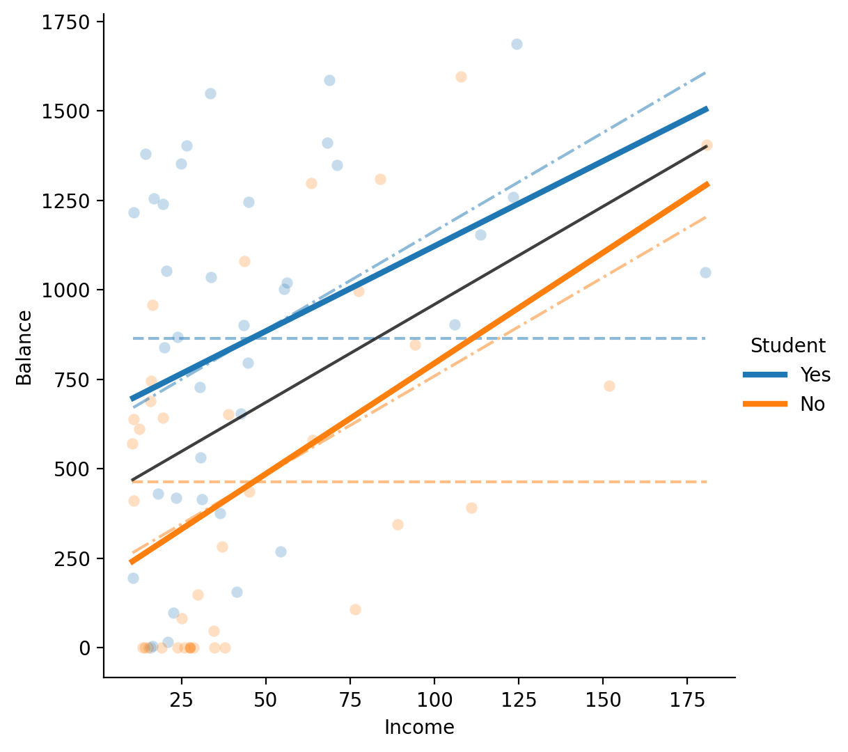
Let’s use the df_models you updated to update our previous figure to see what’s happening visually:

We’ve reduced the opacity of the previous models’ predictions and overlayed the interaction model’s predictions using solid colored lines.

As you can tell, now not only the intercepts are different for each level of Student, but the slopes are also different

# Create grid
grid = sns.FacetGrid(data=df_models.to_pandas(), hue="Student", height=5.5, aspect=1);

# Plot data
grid.map(sns.scatterplot, "Income", "Balance",alpha=.25);

# Plot our predictions from student only model
grid.map(sns.lineplot, "Income", "balance_pred_s", ls='--', alpha=.5);

# Plot our predictions from income only model
grid.map(sns.lineplot, "Income", "balance_pred_i", ls='-', color='black', lw=1.5, alpha=0.5);

# Plot our predictions student + income
grid.map(sns.lineplot, "Income", "balance_pred_si", ls='-.', alpha=.5);

# Plot our predictions student x income
grid.map(sns.lineplot, "Income", "balance_pred_six", lw=3);

# Aesthetics
grid.set(ylabel='Balance');
grid.add_legend();

../../_images/62cfa5d14c4e0af9277af999e39360b9cc8034c0e0b70f31ee46b4d2be38aa7a.png

Let’s inspect the parameter estimates

print(six_results.summary(slim=True))

                            OLS Regression Results                            
==============================================================================
Dep. Variable:                Balance   R-squared:                       0.325
Model:                            OLS   Adj. R-squared:                  0.297
No. Observations:                  76   F-statistic:                     11.57
Covariance Type:            nonrobust   Prob (F-statistic):           2.82e-06
============================================================================================
                               coef    std err          t      P>|t|      [0.025      0.975]
--------------------------------------------------------------------------------------------
Intercept                  176.9471    108.096      1.637      0.106     -38.539     392.434
C(Student)[T.Yes]          470.4184    155.351      3.028      0.003     160.732     780.105
Income                       6.1811      1.765      3.502      0.001       2.662       9.700
C(Student)[T.Yes]:Income    -1.4298      2.584     -0.553      0.582      -6.580       3.721
============================================================================================

Notes:
[1] Standard Errors assume that the covariance matrix of the errors is correctly specified.

Wait we forgot to center! Let’s do that now to make these estimates more interpretable:

six_model_cent = ols('Balance ~ C(Student) * center(Income)', data=df.to_pandas())
six_results_cent = six_model_cent.fit()

print(six_results_cent.summary(slim=True))

                            OLS Regression Results                            
==============================================================================
Dep. Variable:                Balance   R-squared:                       0.325
Model:                            OLS   Adj. R-squared:                  0.297
No. Observations:                  76   F-statistic:                     11.57
Covariance Type:            nonrobust   Prob (F-statistic):           2.82e-06
====================================================================================================
                                       coef    std err          t      P>|t|      [0.025      0.975]
----------------------------------------------------------------------------------------------------
Intercept                          461.4512     70.721      6.525      0.000     320.472     602.430
C(Student)[T.Yes]                  404.6055    100.014      4.045      0.000     205.231     603.980
center(Income)                       6.1811      1.765      3.502      0.001       2.662       9.700
C(Student)[T.Yes]:center(Income)    -1.4298      2.584     -0.553      0.582      -6.580       3.721
====================================================================================================

Notes:
[1] Standard Errors assume that the covariance matrix of the errors is correctly specified.

Let’s verify that:

$\beta_0$ = $\hat{balance}_{\text{student\_no}}$ when $Income = Income_{mean}$
$\beta_1$ = $\hat{balance}_{\text{student\_yes}}$ - $\hat{balance}_{\text{student\_no}}$ when $Income = Income_{mean}$

just like we did before by generating a single marginal prediction

# Create 1-row dataframes to pass into .predict()
student_no_x =pl.DataFrame({
    'Income': df['Income'].mean(),
    'Student': 'No'
})

student_yes_x =pl.DataFrame({
    'Income': df['Income'].mean(),
    'Student': 'Yes'
})

# Generate predictions
student_no_prediction = six_results.predict(student_no_x.to_pandas())
student_yes_prediction = six_results.predict(student_yes_x.to_pandas())

print(f"Student (No): {student_no:.3f}")
print(f"Student (Yes): {student_yes:.3f}")

print(f"Student (No prediction): {student_no_prediction[0]:.3f}")
print(f"Student (Yes prediction): {student_yes_prediction[0]:.3f}")

print(f"Student (Yes prediction - No prediction): {student_yes_prediction[0] - student_no_prediction[0]:.3f}")

Student (No): 463.237
Student (Yes): 864.684
Student (No prediction): 461.451
Student (Yes prediction): 866.057
Student (Yes prediction - No prediction): 404.606

six_results_cent.params

Intercept                           461.451226
C(Student)[T.Yes]                   404.605544
center(Income)                        6.181137
C(Student)[T.Yes]:center(Income)     -1.429850
dtype: float64

To verify that:

$\beta_2$ = $Balance \sim Income$ when $Student =0$
$\beta_3$ = the difference between $Balance \sim Income$ when $Student =0$ vs $Student = 1$

we’ll use the same approach we did in 03_models - we’ll set Student = 0 and Student = 1 and provide the original values for Income to generate marginal predictions for Balance.

Then we’ll estimate the slope of the relationship between these marginal predictions and our original values of Income using 2 univariate regressions:

# Get only student = yes or student = No
student_0_data = df.filter(col('Student') == 'No').select(['Income', 'Student']) 
student_1_data = df.filter(col('Student') == 'Yes').select(['Income', 'Student']) 

# Use values to get model predictions for Balance separately for students and non-students
student_0_predictions = six_results.predict(student_0_data.to_pandas())
student_1_predictions = six_results.predict(student_1_data.to_pandas())

# Create a new dataframe of Predicted_Balance ~ Income when Student = No
marginal_data_student_0 = pl.DataFrame({
    'Income': student_0_data['Income'].to_numpy(),
    'Predicted_Balance': student_0_predictions.to_numpy()
})

# Run univariate OLS to slope
marginal_student_0_params = ols('Predicted_Balance ~ Income', 
                                marginal_data_student_0.to_pandas()).fit().params

# Same for student = Yes
marginal_data_student_1 = pl.DataFrame({
    'Income': student_1_data['Income'].to_numpy(),
    'Predicted_Balance': student_1_predictions.to_numpy()
})

marginal_student_1_params = ols('Predicted_Balance ~ Income', 
                                marginal_data_student_1.to_pandas()).fit().params

print(f"Income slope for Student = No (0): {marginal_student_0_params['Income']:.4f}")
print(f"Income slope for Student = Yes (1): {marginal_student_1_params['Income']:.4f}")

print(f"Difference in slopes: {marginal_student_1_params['Income'] - marginal_student_0_params['Income']:.4f}")

Income slope for Student = No (0): 6.1811
Income slope for Student = Yes (1): 4.7513
Difference in slopes: -1.4298

And we can see the interaction term reflects this difference-in-slopes while center(Income) reflects the slope of Student = No

six_results_cent.params

Intercept                           461.451226
C(Student)[T.Yes]                   404.605544
center(Income)                        6.181137
C(Student)[T.Yes]:center(Income)     -1.429850
dtype: float64

Summary#

When we multiply a categorical predictor in a model with a continuous predictor, we estimate different intercepts and different slopes for each level of the categorical variable.

Intuitively, this is like fitting a separate univariate regression to each level of the categorical variable and comparing the difference-in-slopes of both regressions.

Alternatively, we can think about it testing whether the mean difference between levels of our categorical variable increase or decrease as we move along the continuous predictor.

Centering our continuous predictor makes our estimates more interpretable. It also makes sure we compare levels of our categorical predictor along a meaningful value of our continuous predictor!

Challenge#

In the Parameter Interpretation section of 03_models we had you answer a response challenge about a model you built using the advertising dataset:

\[ sales_i = \beta_0 + \beta_1 tv_i + \beta_2 radio_i \]

Specifically we said:

Notice in the plot above that the slopes of the predicted lines are not changing - it looks like only the intercept is shifting up or down. Can you provide an explanation why? What is our model failing to capture and how might we fix this?

Your tasks#

Using what you learned about interactions in multiple regression:

Estimate the model using the formula above (same as in 03_models)
Estimate a new model that captures what this model is missing
Compare this new model to the original model to see if it’s worth it
Make a new figure like the one above that visualizes the predictions from your new model
Interpret the parameter estimates from .summary() and provide a natural-language explanation of what they mean
Fit another like you just did, but this time center each predictor
How are the parameter estimates from this model different to the uncentered one?
Compare the correlations between predictors in the centered and uncentered models using the provided function

Variable	Description
tv	TV ad spending in $1000 of dollars
radio	Radio ad spending in $1000 of dollars
newspaper	Newspaper ad spending in $1000 of dollars
sales	Sales generated in $1000 of dollars

import numpy as np
import polars as pl
from polars import col
import seaborn as sns
import matplotlib.pyplot as plt
from statsmodels.formula.api import ols
df = pl.read_csv('./data/advertising.csv')
df.head()

shape: (5, 4)

tv	radio	newspaper	sales
f64	f64	f64	f64
230.1	37.8	69.2	22.1
44.5	39.3	45.1	10.4
17.2	45.9	69.3	9.3
151.5	41.3	58.5	18.5
180.8	10.8	58.4	12.9

1) Estimate model from previous notebook#

# Solution
model_c = ols('sales ~ tv + radio', data=df.to_pandas())
results_c = model_c.fit()

2) Estimate new model#

# Solution
model_a = ols('sales ~ tv + radio + tv:radio', data=df.to_pandas())
results_a = model_a.fit()

3) Compare both models#

# Solution
anova_lm(results_c, results_a)

	df_resid	ssr	df_diff	ss_diff	F	Pr(>F)
0	197.0	556.913980	0.0	NaN	NaN	NaN
1	196.0	174.483383	1.0	382.430597	429.590463	2.757681e-51

4) Figure of model predictions#

# Solution
# Save to variable just to make coding easier
tv = df['tv'].to_numpy()
zeros = np.repeat(0, len(tv))
twenty = np.repeat(20, len(tv))
forty = np.repeat(40, len(tv))

# We use all values in the TV column
# And just a bunch of 0s for radio
y_radio_0 = results_a.predict({'tv': tv, 'radio': zeros, 'tv:radio':tv * zeros})
y_radio_20 = results_a.predict({'tv': tv, 'radio': twenty, 'tv:radio':tv * twenty})
y_radio_40 = results_a.predict({'tv': tv, 'radio': forty, 'tv:radio':tv * forty})

grid = sns.relplot(
    data=df,
    kind='scatter',
    x='tv',
    y='sales',
    hue='radio',
    size='radio',

)
grid.set(xlabel='TV Spending ($1000)', ylabel='Sales ($1000)');
grid.legend.set_title('Radio Spending ($1000)');
grid.legend.set_bbox_to_anchor((.45, .8));

# Add them to the plot
grid.ax.plot(tv, y_radio_0, color='gray');
grid.ax.plot(tv, y_radio_20, color='gray');
grid.ax.plot(tv, y_radio_40, color='gray');

5) Interpret parameter estimates#

# Solution
print(results_a.summary())

                            OLS Regression Results                            
==============================================================================
Dep. Variable:                  sales   R-squared:                       0.968
Model:                            OLS   Adj. R-squared:                  0.967
Method:                 Least Squares   F-statistic:                     1963.
Date:                Tue, 18 Feb 2025   Prob (F-statistic):          6.68e-146
Time:                        16:12:39   Log-Likelihood:                -270.14
No. Observations:                 200   AIC:                             548.3
Df Residuals:                     196   BIC:                             561.5
Df Model:                           3                                         
Covariance Type:            nonrobust                                         
==============================================================================
                 coef    std err          t      P>|t|      [0.025      0.975]
------------------------------------------------------------------------------
Intercept      6.7502      0.248     27.233      0.000       6.261       7.239
tv             0.0191      0.002     12.699      0.000       0.016       0.022
radio          0.0289      0.009      3.241      0.001       0.011       0.046
tv:radio       0.0011   5.24e-05     20.727      0.000       0.001       0.001
==============================================================================
Omnibus:                      128.132   Durbin-Watson:                   2.224
Prob(Omnibus):                  0.000   Jarque-Bera (JB):             1183.719
Skew:                          -2.323   Prob(JB):                    9.09e-258
Kurtosis:                      13.975   Cond. No.                     1.80e+04
==============================================================================

Notes:
[1] Standard Errors assume that the covariance matrix of the errors is correctly specified.
[2] The condition number is large, 1.8e+04. This might indicate that there are
strong multicollinearity or other numerical problems.

6) Fit a model with centered predictors#

# Solution
model_a_cent = ols('sales ~ center(tv) * center(radio)', data=df.to_pandas())
results_a_cent = model_a_cent.fit()

print(results_a_cent.summary(slim=True))

                            OLS Regression Results                            
==============================================================================
Dep. Variable:                  sales   R-squared:                       0.968
Model:                            OLS   Adj. R-squared:                  0.967
No. Observations:                 200   F-statistic:                     1963.
Covariance Type:            nonrobust   Prob (F-statistic):          6.68e-146
============================================================================================
                               coef    std err          t      P>|t|      [0.025      0.975]
--------------------------------------------------------------------------------------------
Intercept                   13.9470      0.067    208.737      0.000      13.815      14.079
center(tv)                   0.0444      0.001     56.673      0.000       0.043       0.046
center(radio)                0.1886      0.005     41.806      0.000       0.180       0.198
center(tv):center(radio)     0.0011   5.24e-05     20.727      0.000       0.001       0.001
============================================================================================

Notes:
[1] Standard Errors assume that the covariance matrix of the errors is correctly specified.
[2] The condition number is large, 1.28e+03. This might indicate that there are
strong multicollinearity or other numerical problems.

7) How are the parameter estimates from centered and un-centered models the same or different?#

Uncentered predictor slopes assume other predictors = 0
Centered predictor slopes assume other predictors = their respective means

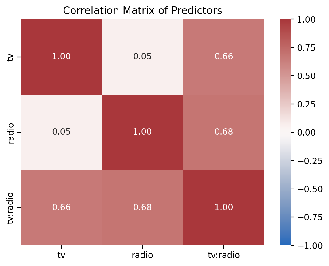
8) Compare the correlations between centered and un-centered models#

Use the provided function plot_predictor_correlations to visualize the correlation matrix of the predictors for both the centered and uncentered models.

Then answer the question below

from helpers import plot_predictor_correlations

# Example Usage
# plot_predictor_correlations(my_model)

# Solution
ax = plot_predictor_correlations(model_a)

../../_images/fee5a942fe75d6da03a5811ccf1cf19caef4d1aa371c3ab5cefd76248d0bac53.png

# Solution
ax = plot_predictor_correlations(model_a_cent)

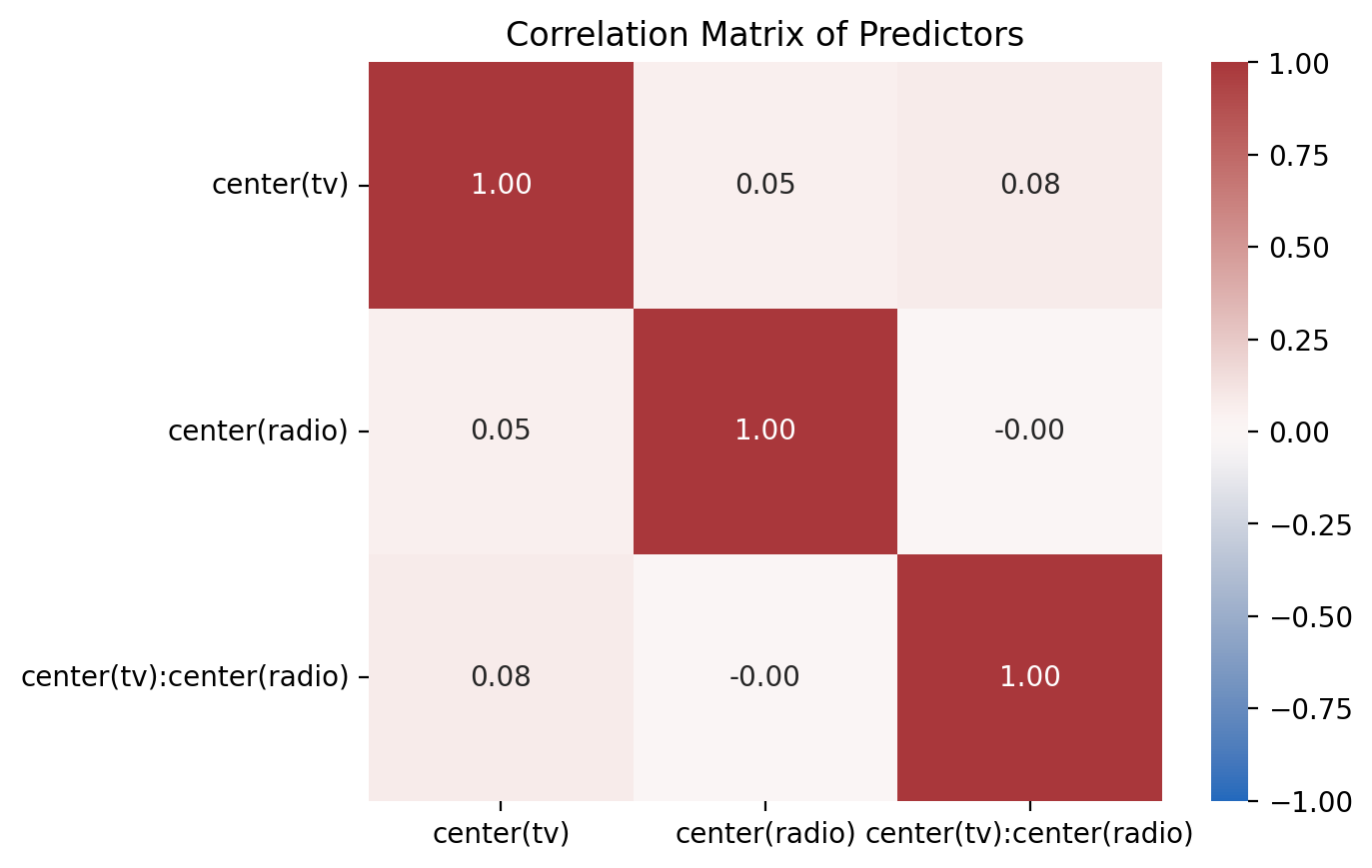
../../_images/80a60b01ba78207c13afc73ff03e0e4c82df19bd8fc0b5f3600e5cb63051ab9b.png

How do you think the change in correlation will affect our estimates and inferences?

Your response here

Models V: Categorical Predictors (2-levels)

Contents

Models V: Categorical Predictors (2-levels)#

Slides for reference#

Data#

Categorical Predictor w/ 2 levels#

Introduction to Categorical Coding Schemes#

Treatment (Dummy) Coding#

Challenge#

Interpreting parameter estimates#

Categorical (2-level) and Continuous Predictors#

Challenge#

Interpreting Parameter Estimates#

Challenge#

Visualizing intutions#

Summary#

Interactions (2-levels and Continuous Predictor)#

Challenge#

Interpreting Parameter Estimates#

Summary#

Challenge#

Your tasks#

1) Estimate model from previous notebook#

2) Estimate new model#

3) Compare both models#

4) Figure of model predictions#

5) Interpret parameter estimates#

6) Fit a model with centered predictors#

7) How are the parameter estimates from centered and un-centered models the same or different?#

8) Compare the correlations between centered and un-centered models#