Linear Mixed Models II: LMMs with Categorical Predictors

Important (if you didn’t do this before trying out 01_lmms):
Before running this notebook open a terminal, activate the 201b environment, and update the pymer4 package:

1. Open terminal

2. conda activate 201b

3. pip install git+https://github.com/ejolly/pymer4.git --no-deps

Learning Goals & Resources

In the previous notebook we got a general introduction to Linear Mixed Models (LMMs) and met the pymer4 library. In this notebook we’ll build upon that foundation and focus on:

• Exploring the challenge solution from 01_lmms

• How to decide your random-effect structure

• Interpreting model output

• LMMs with categorical predictor (2 levels)

• LMMs with categorical predictor (3 levels)

• Post-hoc tests of categorical predictors

Slides for reference

Linear Mixed Models I (slides from 03-10)

Excellent Resources

We’ve compiled a list of excellent resources to better help you understand LMMs and posted it to the course website at this URL: https://tinyurl.com/lmm-resources

Review

Let’s begin by reviewing the interactive visual explainer from yesterday:

http://mfviz.com/hierarchical-models/

# Import some libraries we typically use
import matplotlib.pyplot as plt
import seaborn as sns
import numpy as np
import polars as pl
from polars import col
sns.set_context('notebook')
df = pl.read_csv('data/sleep.csv')

How do I decide what my random effects are? (solution from 01_lmms)

Let’s review the challenge question from the end of the previous notebook. What this question is really getting after is helping you think about how to decide what random effects to use.

This is a different question than what effects are significant and should be the first step in your LMM model-building process. What we’re after is understanding:

• How much variability is there amongst my repeated measurements?

• Does taking this variability into account fit the data better?

We’re going to take the approach we learned about in class: use the Maximal random-effects structure supported by your design and data

Let’s start by building 3 models with 3 different random-effect structures from the end of the previous notebook and using model comparison:

1. Random intercepts only: accounts for baseline Reaction differences amongst Subjects

2. Random slopes only: accounts for differences in the effect of Days amongst Subjects

3. Random intercepts + slopes: accounts for both baseline differences and effect differences (maximal model)

As a reminder here’s the data:

Variable	Description
Subject	Unique Subject ID
Days	Number of Days of sleep deprivation
Reaction	Subject’s Reaction time in ms

from pymer4.models import Lmer

# Random intercepts
model_i = Lmer('Reaction ~ Days + (1 | Subject)', data=df.to_pandas())
model_i.fit()

# Random slopes
model_s = Lmer('Reaction ~ Days + (0 + Days | Subject)', data=df.to_pandas())
model_s.fit()

# Random intercepts + slopes (correlated)
model_is = Lmer('Reaction ~ Days + (1 + Days | Subject)', data=df.to_pandas())
model_is.fit()

Model comparison

To compare these models we can use the lrt() function which calculates a likelihood-ratio test between models
This allows us to ask the same question we’ve been asking when we compared ols() models using anova_lm():

Do the additional model parameters result in a meaningful reduction in error (or improvement in fit)?

The output below shows us that there isn’t much difference between using only random intercepts or only random slopes. But the addition of both random intercepts and random slopes is worth it! In this case we’re going to stick with our maximal model

from pymer4.stats import lrt

lrt(model_i, model_s, model_is)

refitting model(s) with ML (instead of REML)

	model	npar	AIC	BIC	log-likelihood	deviance	Chisq	Df	P-val	Sig
0	Reaction~Days+(1|Subject)	4	1802.078643	1814.850470	-897.039322	1794.078643
1	Reaction~Days+(0+Days|Subject)	4	1782.080315	1794.852143	-887.040158	1774.080315	19.998328	0.0
2	Reaction~Days+(1+Days|Subject)	6	1763.939344	1783.097086	-875.969672	1751.939344	22.140971	2.0	0.000016	***

Examine estimated variance across clusters

Let’s take a look at the estimated random-effects variance for our maximal model. We can do this by using the .ranef_var attribute of our model
Each row is a random-effect we estimated and the columns are variance and standard deviation

model_is.ranef_var

	Name	Var	Std
Subject	(Intercept)	612.100158	24.740658
Subject	Days	35.071714	5.922138
Residual		654.940008	25.591796

We can see that there is indeed quite a bit of variability across Subject intercepts (SD = 24.74) and Subject sopes (SD = 5.92)
Let’s try to visualize this, but first let’s remind ourselves of what the LMM equation looks like:

\[Reaction_{ij} = (\beta_0 + b_{0j}) + (\beta_1 + b_{1j})Days_{ij} + \epsilon_{ij}\]

Term	Code	Part of the Model	Description
\(\beta_0\)	model.coef	fixed	the grand intercept (mean Reaction when Days is 0)
\(\beta_1\)	model.coef	fixed	the grand slope (effect of Days)
\(b_{0j}\)	model.ranef	random	subject \(\text{j's}\) deviance from grand intercept
\(b_{1j}\)	model.ranef	random	subject \(\text{j's}\) deviance from grand slope
\(\beta_0 + b_{0j}\)	model.fixef	estimated BLUP	subject \(\text{j's}\) estimated intercept
\(\beta_1 + b_{1j}\)	model.fixef	estimated BLUP	subject \(\text{j's}\) estimated slope

Models estimated with Lmer() store each part of the LMM equation as separate attributes noted in the Code column of the table. To visualize the variability across people we’ll take a look at each subject’s BLUP: Best Linear Unbiased Ppredictor

This is stored in the .fixef attribute

Remember our LMM doesn’t estimate these directly! Instead it estimates how much random-effect (i.e. Subject’s intercept or slope) deviates from the fixed effects (i.e. overall intercept and slope). Lmer() automatically calculates these for you and stores them in pandas DataFrame

Below each row is a Subject and the columns are their BLUPs, parameter estimates for intercept and slope:

model_is.fixef

	(Intercept)	Days
308	253.663656	19.666262
309	211.006367	1.847605
310	212.444696	5.018429
330	275.095724	5.652936
331	273.665417	7.397374
332	260.444673	10.195109
333	268.245613	10.243650
334	244.172490	11.541868
335	251.071436	-0.284879
337	286.295592	19.095551
349	226.194876	11.640718
350	238.335071	17.081504
351	255.982969	7.452024
352	272.268783	14.003287
369	254.680570	11.339501
370	225.792106	15.289771
371	252.212151	9.479130
372	263.719697	11.751308

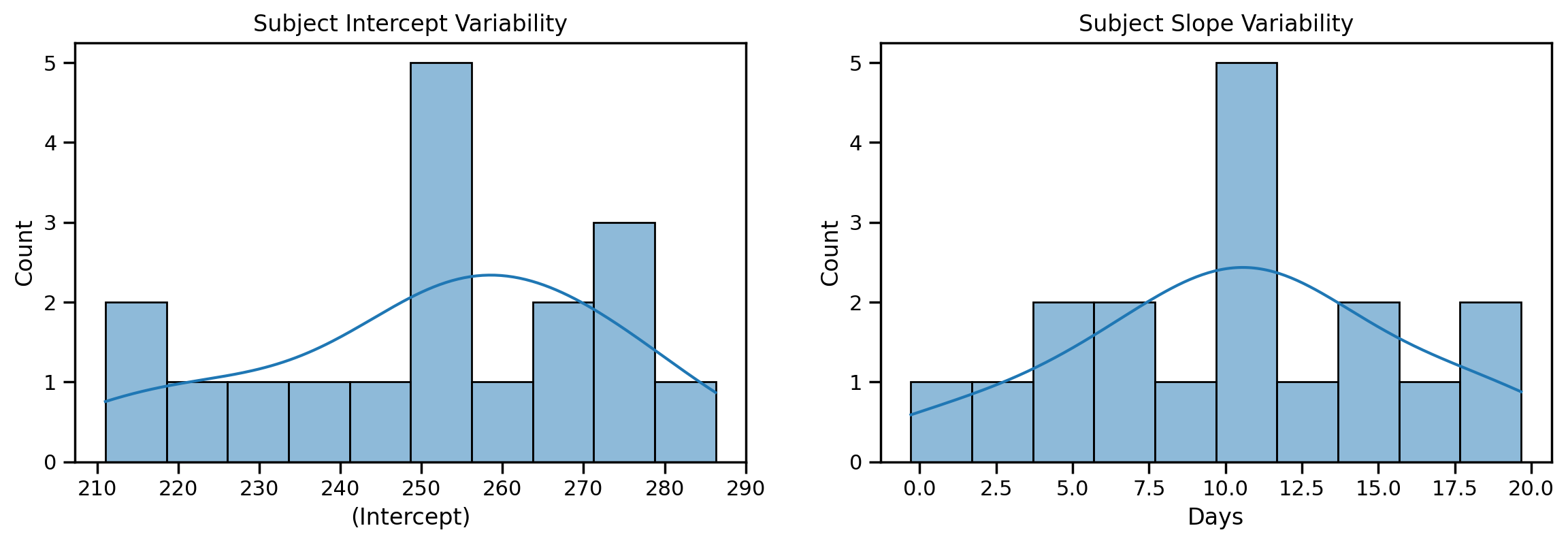
Let’s use these to make 2 histograms that visualize the spread across people.

On the left you can see the variability across each person’s average Reaction when Days = 0; some people responded as quickly as 210ms on average, whereas others more like 280ms.

On the right you can see how the effect of Days varied by person, from a range of almost no effect up to a nearly 20ms increase in RT for each additional Day of sleep deprivation:

f, axs = plt.subplots(1,2, figsize=(14,4))

# Intercept
ax = sns.histplot(model_is.fixef['(Intercept)'], kde=True, bins=10, ax=axs[0])
ax.set_title('Subject Intercept Variability')

# Slope
ax = sns.histplot(model_is.fixef['Days'], kde=True, bins=10, ax=axs[1])
ax.set_title('Subject Slope Variability');

Let’s say we didn’t take the varibility of Days across people into account. What would happen to our statistical inferences?
Remember we learned that our Type I error-rate would increase! We would be more likely to report a false positive result

We can see how ignoring this variability puts us in this situation by comparing the standard error of our fixed effects between models with and without a random slope. Notice how for the first model (random intercept only) the estimated SE for Days is about 0.80 which results a t-statistic of nearly 13.02. That’s huge t-stat with commensurately tiny p-value!

model_i.coefs

	Estimate	2.5_ci	97.5_ci	SE	DF	T-stat	P-val	Sig
(Intercept)	251.405105	232.301892	270.508318	9.746716	22.810199	25.793826	2.241351e-18	***
Days	10.467286	8.891041	12.043531	0.804221	161.000000	13.015428	6.412601e-27	***

Now look at the SE for Days in the model with both random intercepts & random slopes. See how it’s nearly 2x larger? This results in a t-statistic that almost half our previous one 13.02 -> 6.77!

model_is.coefs

	Estimate	2.5_ci	97.5_ci	SE	DF	T-stat	P-val	Sig
(Intercept)	251.405105	238.029141	264.781069	6.824597	16.999726	36.838090	1.171558e-17	***
Days	10.467286	7.437594	13.496978	1.545790	16.999984	6.771481	3.263824e-06	***

Because there’s a real effect in these data, our estimated coefficent doesn’t really change (10.467). But, by asking our model to incorporate the variability across how sleep deprivation affects each person differently, we become a little more uncertain of our estimate, and a therefore a little more cautious before we reject the null hypothesis.

So how do I decide?

In summary we recommend the following approach:

1. Always start with the maximal model you can estimate

2. If you see warnings or errors when calling .fit() simplify by removing random-effects

• Start with correlation between intercept and slope (see formula table from 01_lmms or below)

• Then remove slopes

• Lastly consider removing intercepts

3. Always examine the variability across your clusters using .ranefor visually

4. Use lrt() to perform model comparison

5. Finally once you’ve decided on the your random effects, then and only then interpret the inferences on your fixef effects (.coef)

Challenge

Use the formula syntax examples below to estimate an LMM with uncorrelated intercepts and slopes.

Compare it to model_is which includes intercepts, slopes, and their correlation. What do you notice?

Your response here

# Solution
model_is_nocorr = Lmer('Reaction ~ Days + (1 | Subject) + (0 + Days | Subject)', data=df.to_pandas())
model_is_nocorr.fit()

lrt(model_is, model_is_nocorr)

refitting model(s) with ML (instead of REML)

	model	npar	AIC	BIC	log-likelihood	deviance	Chisq	Df	P-val	Sig
0	Reaction~Days+(1|Subject)+(0+Days|Subject)	5	1762.003255	1777.968039	-876.001628	1752.003255
1	Reaction~Days+(1+Days|Subject)	6	1763.939344	1783.097086	-875.969672	1751.939344	0.063911	1.0	0.800418

Better understanding the output

Let’s take a look at the summary that Lmer() models give us. We can get this in one of two ways:

• By passing summarize = True to .fit()

• Using the .summary() method anytime after you’ve used .fit()

The first part of the summary tells us some basic information about the model, our data, and how Lmer() interpreted and estimated the random-effects we asked for, including:

• the number of observations (180)

• the number of clusters (Groups) 18

• Log-likelihood & AIC - statistics that reflect the overall fit of the model and let us compare it to other models

• the variance-covariance of our random-effects (intercept, slope, and their correlation)

• the fixed effects which looks similar to the output when we summarize an ols model

Remember we interpret these estimates the same way we would for standard GLM models: the unit change in Y for each unit change in X, assuming all other predictors in the model = 0

model_is.summary()

Linear mixed model fit by REML [’lmerMod’]
Formula: Reaction~Days+(1+Days|Subject)

Family: gaussian	 Inference: parametric

Number of observations: 180	 Groups: {'Subject': 18.0}

Log-likelihood: -871.814 	 AIC: 1755.628

Random effects:

                 Name      Var     Std
Subject   (Intercept)  612.100  24.741
Subject          Days   35.072   5.922
Residual               654.940  25.592

                 IV1   IV2   Corr
Subject  (Intercept)  Days  0.066

Fixed effects:

	Estimate	2.5_ci	97.5_ci	SE	DF	T-stat	P-val	Sig
(Intercept)	251.405	238.029	264.781	6.825	17.0	36.838	0.0	***
Days	10.467	7.438	13.497	1.546	17.0	6.771	0.0	***

If we look at the output of our model with only random intercepts we can see that the slope and correlation are missing the in Random Effects of the summary:

model_i.summary()

Linear mixed model fit by REML [’lmerMod’]
Formula: Reaction~Days+(1|Subject)

Family: gaussian	 Inference: parametric

Number of observations: 180	 Groups: {'Subject': 18.0}

Log-likelihood: -893.233 	 AIC: 1794.465

Random effects:

                 Name       Var     Std
Subject   (Intercept)  1378.179  37.124
Residual                960.457  30.991

No random effect correlations specified

Fixed effects:

	Estimate	2.5_ci	97.5_ci	SE	DF	T-stat	P-val	Sig
(Intercept)	251.405	232.302	270.508	9.747	22.81	25.794	0.0	***
Days	10.467	8.891	12.044	0.804	161.00	13.015	0.0	***

A topic of some debate in the LMM literature is how to best calculate p-values. There reason for this is because the lme4 R package (upon which pymer4 is based) does not include p-values by default

Remember we can always using model comparison with and without fixed effects terms to achieve a similar inference.

• For Lmer() models we do this with the lrt() function, not only to compare random-effects but also fixed effects.

• For ols() models we do this using the anova_lm() function and we only have fixed effects in these types of models.

A popular alternative that controls false postive rates well is using Satterthwaite or Kenward-Roger approximation to calculate degrees-of-freedom that account for the dependent structure of our model. These allow us to perform parametric inference just like we’re familiar with:

• Estimate t-stat using ratio of coefficient to standard-error and use degrees-of-freedom to look up p-value assuming a t-distribution

This is the approach that Lmer() automatically performs for you and includes in the summary output using the popular lmerTest package. However, this is a semi-controversial issue in the literature so we’ll leave you with the core help page in R with recommendations:

• Why doesn’t lme4 display dof or p-values?

• Getting p-values for fitted models (screenshot below)

Categorical Predictor with 2-levels (paired t-test)

Just like with ols() models we can also using categorical predictors in Lmer() models.

Let’s load some simulated data from 20 participants who provided responses to 2 conditions that we want to compare. This is repeated measures design because every participant responded to both conditions.

Let’s load the data and visualize each participant in a different color:

df2 = pl.read_csv('data/2levels.csv')
df2.head()

shape: (5, 3)

participant	condition	value
i64	str	f64
1	"A"	1.624345
2	"A"	-0.611756
3	"A"	-0.528172
4	"A"	-1.072969
5	"A"	0.865408

order = ['A', 'B']
grid = sns.FacetGrid(data=df2.to_pandas(), hue='participant', height=4)
grid.map(sns.lineplot, 'condition', 'value')
grid.map(sns.pointplot, 'condition', 'value', order=order);

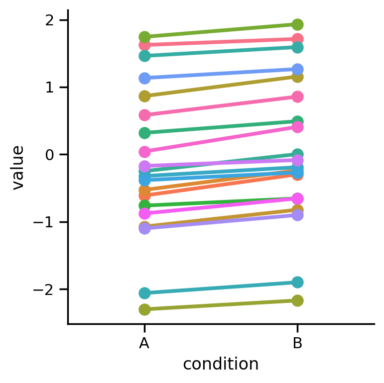
We can see that difference between conditions is small but consistent across all our participants. We can use seaborn to visualize the means of each condition and calculate 95% CIs that either ignore the dependence in the data or include the dependence in the data.

If we include the dependence our CIs are wider on average (orange wider than blue). This is consistent with the increase of the standard-error we saw earlier. We’re a little more uncertain about our estimate when we take into account the dependency.

sns.pointplot(x='condition', y='value', data=df2.to_pandas(), label='ignore dependence', seed=1)
sns.pointplot(x='condition', y='value', units='participant', color='orange', alpha=.6, data=df2.to_pandas(), label='include dependence', seed=0)
sns.despine();

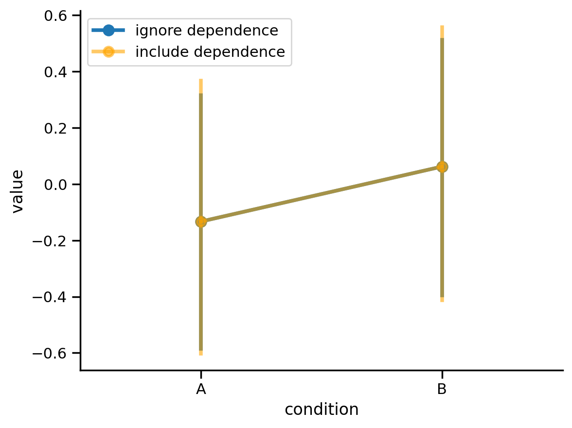
However, ignoring dependency doesn’t always mean a Type I error (false positive). Sometimes it means a Type II error (false negative)

In this case even though the effect is small, it’s consistent across every single person.

Let’s see what happens if we fit a regular ‘ol ols() aka use complete pooling. Remember to specificy a categorical variable in an ols() model we wrap it in C()

from statsmodels.formula.api import ols
lm = ols('value ~ C(condition)', data=df2.to_pandas()).fit()
print(lm.summary(slim=True))

                            OLS Regression Results                            
==============================================================================
Dep. Variable:                  value   R-squared:                       0.008
Model:                            OLS   Adj. R-squared:                 -0.018
No. Observations:                  40   F-statistic:                    0.3002
Covariance Type:            nonrobust   Prob (F-statistic):              0.587
=====================================================================================
                        coef    std err          t      P>|t|      [0.025      0.975]
-------------------------------------------------------------------------------------
Intercept            -0.1334      0.252     -0.529      0.600      -0.644       0.377
C(condition)[T.B]     0.1954      0.357      0.548      0.587      -0.527       0.917
=====================================================================================

Notes:
[1] Standard Errors assume that the covariance matrix of the errors is correctly specified.

We can see that this difference is not statistically significant and that our standard-error is quite large (0.357) producing a small t-statistic (0.548)

This analysis assumes that each condition was experience by entirely independent groups of participants.

In fact it’s exactly the same as an independent-samples t-test:

# t-test function from scipy
from scipy.stats import ttest_ind

# values in condition A
condA = df2.filter(col('condition') == 'A')['value'].to_numpy()

# values in condition B
condB = df2.filter(col('condition') == 'B')['value'].to_numpy()

t, pval = ttest_ind(condB, condA)
print(f"t = {t:.3f}, p = {pval:.4f}")

t = 0.548, p = 0.5869

Let’s see what happens when we fit an LMM to account for the dependency between conditions, which we can do by adding a random intercept per participant.
Specifying categorical variables in Lmer() models uses different syntax from ols()

For Lmer() models, we don’t use C() in the model formula.
Instead we use the factors={} argument to .fit() and provide it a dictionary ({}) of contrasts.

• The key of the dictionary is the name of each of our categorical variables 'condition' in this case

• The value of the dictionary is list of the levels of our categorical variable, with the first level being set as the reference level.

• This is equivalent to the default contrasts that C() creates in ols() models: dummy/treatment coding

In the code below since condition A comes first, it will be used as the model intercept and the parameter estimate reflects the difference between condition B - condition A

For additional details you can check out the tutorial on the pymer4 website

lmm = Lmer('value ~ condition + (1 | participant)', data=df2.to_pandas())

lmm.fit(factors={
    'condition': ['A', 'B'] # A will be intercept and parameter is B-A
})

If we inspect the summary, we can see the effect is now significant! Why? Take a look at our standard-error…

Beause the effect is consistent across every participant, it reduces our uncertainty and the LMM explicitly models that!
This gives us the correct error calculation, increases our power, and reduces our false negative rate.

lmm.summary()

Linear mixed model fit by REML [’lmerMod’]
Formula: value~condition+(1|participant)

Family: gaussian	 Inference: parametric

Number of observations: 40	 Groups: {'participant': 20.0}

Log-likelihood: -11.797 	 AIC: 31.593

Random effects:

                    Name    Var    Std
participant  (Intercept)  1.269  1.126
Residual                  0.003  0.058

No random effect correlations specified

Fixed effects:

	Estimate	2.5_ci	97.5_ci	SE	DF	T-stat	P-val	Sig
(Intercept)	-0.133	-0.628	0.361	0.252	19.051	-0.529	0.603
condition1	0.195	0.159	0.232	0.018	19.000	10.586	0.000	***

In fact this is the LMM equivalent of a paired-samples t-test:

from scipy.stats import ttest_rel

t, pval = ttest_rel(condB, condA)
print(f"t = {t:.3f}, p = {pval:.4f}")

t = 10.586, p = 0.0000

Categorical Predictor with 3+ levels (rm-ANOVA)

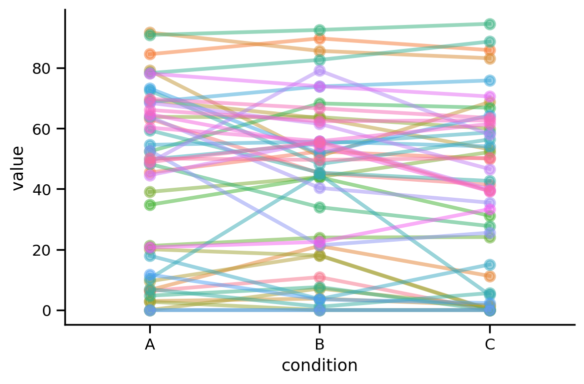
Let’s look at one more example this time using a categorical predictor with 3 levels. Like before these data come from a repeated measures design, where each of 12 participants provided a response to every condition:

3 replicates (observations) per cluster (subject) in LMM lingo

Let’s visualize the data like before and compare what happens when we estimate a standard ols() model (ignoring dependence) and Lmer() that explicitly models it

df3 = pl.read_csv('data/3levels.csv')

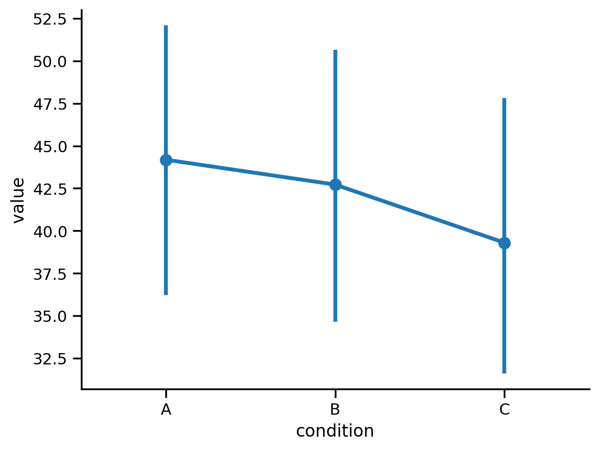
Visually, the effect isn’t as consistent across people as our previous 2-level example data but it does look like there’s a slight downward trend from condition A -> C

order = ['A', 'B', 'C']
grid = sns.FacetGrid(data=df3.to_pandas(), hue='participant', height=4, aspect=1.5)
grid.map(sns.pointplot, 'condition', 'value', order=order, errorbar=None, alpha=0.5);

We can see this reflected in the means, but we don’t know if this is meaningful in light of our uncertainty:

order = ['A', 'B', 'C']
sns.pointplot(x='condition', y='value', order=order, units='participant', data=df3.to_pandas())
sns.despine();

Let’s use ols() to run a one-way ANOVA, ignoring the dependency.

Remember it’s good practice to use an orthogonal coding scheme for valid ANOVA tests.

We can do that using C(variable, Sum) or C(variable, Poly) to use deviation/sum or polynomial coding respectively. Both schemes will produce valid ANOVA results, especially in the face of unbalanced data.

We also want to remember to tell the anova_lm() function to use type III sum-of-squares calculations:

from statsmodels.stats.anova import anova_lm

# Orthogonal polynomial contrasts
lm = ols('value ~ C(condition, Poly)', data=df3.to_pandas()).fit()

# Type 3 SS
anova_lm(lm, typ=3).round(4)

	sum_sq	df	F	PR(>F)
Intercept	998181.7083	1.0	1064.5161	0.0000
C(condition, Poly)	2359.7781	2.0	1.2583	0.2849
Residual	526041.7985	561.0	NaN	NaN

We can see that this result is not significant. Now let’s try estimating an LMM that explicitly models this dependency. We’ll do this again by using random intercepts per participants and use factors to specific condition as a categorical variable.

To perform an F-test we can use the .anova() method which will calculate type III sum-of-squares for us. We will need to ensure we’re using an orthogonal coding scheme for valid F-tests, but Lmer() offers us 2 ways to do so:

1. Use the ordered = True argument to .fit() after you specify your factors

2. Specify whatever you want for factors and pass the force_orthogonal=True argument to .anova()

Both approaches will use the same strategy as C(variable, Poly) by estimating polynomial contrasts that are orthogonal

# Setup model
lmm = Lmer('value ~ condition + (1 | participant)', data=df3.to_pandas())

# Categorical variables
lmm.fit(factors={
    'condition': ['A', 'B', 'C'],
    }, ordered=True) # add ordered = True to ensure orthogonal coding

# Calculate main-effect
lmm.anova()

# Alternatively - but same result
# lmm.anova(force_orthogonal=True)

SS Type III Analysis of Variance Table with Satterthwaite approximated degrees of freedom:
(NOTE: Using original model contrasts, orthogonality not guaranteed)

	SS	MS	NumDF	DenomDF	F-stat	P-val	Sig
condition	2359.778135	1179.889067	2	515.000001	5.296284	0.005287	**

Accounting for the dependence means makes our result significant!
We can see how by inspecting the coefficients and their uncertainties like before.
Compared to the output of our ols() model our standard errors are again smaller thus resulting in less uncertainty about our estimates:

print(lm.summary(slim=True))

                            OLS Regression Results                            
==============================================================================
Dep. Variable:                  value   R-squared:                       0.004
Model:                            OLS   Adj. R-squared:                  0.001
No. Observations:                 564   F-statistic:                     1.258
Covariance Type:            nonrobust   Prob (F-statistic):              0.285
================================================================================================
                                   coef    std err          t      P>|t|      [0.025      0.975]
------------------------------------------------------------------------------------------------
Intercept                       42.0693      1.289     32.627      0.000      39.537      44.602
C(condition, Poly).Linear       -3.4518      2.233     -1.546      0.123      -7.838       0.935
C(condition, Poly).Quadratic    -0.7984      2.233     -0.357      0.721      -5.185       3.588
================================================================================================

Notes:
[1] Standard Errors assume that the covariance matrix of the errors is correctly specified.

Remember because we’ve used a polynomial coding scheme the first parameter below condition1 represents a linear trend across conditions and the second parameter condition2 represents a quadratic trend across conditions

We can interpret these the same as the C(condition, Poly).Linear and C(condition.Poly).Quadratic that we see in the ols output above

lmm.summary()

Linear mixed model fit by REML [’lmerMod’]
Formula: value~condition+(1|participant)

Family: gaussian	 Inference: parametric

Number of observations: 564	 Groups: {'participant': 47.0}

Log-likelihood: -2405.782 	 AIC: 4821.564

Random effects:

                    Name      Var     Std
participant  (Intercept)  726.565  26.955
Residual                  222.777  14.926

No random effect correlations specified

Fixed effects:

	Estimate	2.5_ci	97.5_ci	SE	DF	T-stat	P-val	Sig
(Intercept)	42.069	34.265	49.873	3.982	46.0	10.566	0.000	***
condition1	-3.452	-5.585	-1.318	1.089	515.0	-3.171	0.002	**
condition2	-0.798	-2.932	1.335	1.089	515.0	-0.733	0.464

Post-hoc comparisons

Our LMM summary suggests that there’s a linear trend across conditions. Which conditions?
We can perform follow-up post-hoc comparisons like we learned about for ols() models using the marginaleffects package.

For Lmer() models the syntax is different and a bit easier to work with: we just use the .post_hoc() method and pass in the name(s) of the marginal_vars we want to calcualte ANOVA-style cell-means and comparisons for.

We can also use the p_adjust argument to correct for multiple comparisons.

Let’s look at the means and comparisons between each condition and adjust for multiple comparisons using FDR.

Note Lmer() also supports more complicated categorical designs (e.g. two-way ANOVA, ANCOVA). You can control post-hoc tests for these designs by passing in additional marginal_vars or by using grouping_vars. See the pymer4 website for more details and examples

# Calculate means for each level of 'condition' and compare them pair-wise with fdr correction
means, comparisons = lmm.post_hoc(marginal_vars='condition', p_adjust='fdr')

P-values adjusted by fdr method for 3 comparisons

means

	condition	Estimate	2.5_ci	97.5_ci	SE	DF
1	A	44.184	35.993	52.376	4.08	50.687
2	B	42.721	34.530	50.913	4.08	50.687
3	C	39.303	31.111	47.494	4.08	50.687

Our pairwise comparisons show us that the difference between condition A and the other 2 conditions seems to be the driving factor in our omnibus F-test

comparisons

	Contrast	Estimate	2.5_ci	97.5_ci	SE	DF	T-stat	P-val	Sig
1	A - B	1.463	-2.235	5.160	1.539	515.0	0.950	0.342
2	A - C	4.882	1.184	8.579	1.539	515.0	3.171	0.005	**
3	B - C	3.419	-0.279	7.116	1.539	515.0	2.221	0.040	*

Interpreting categorical random-effects

Let’s wrap up by exploring how LMMs handle categorical random-effects
In short: they use the same encoding for fixed and random effects.

Let’s see his by estimating random slopes across condition for each of our participants:

# Setup model
lmm_with_slopes = Lmer('value ~ condition + (condition | participant)', data=df3.to_pandas())

# Categorical variables
lmm_with_slopes.fit(factors={
    'condition': ['A', 'B', 'C'],
    }, ordered=True) # add ordered = True to ensure orthogonal coding

boundary (singular) fit: see help('isSingular') 

Let’s ignore that warning for now. We know that for our fixed effects the polynomial coding scheme will estimate a linear trend and a quadratic trend, which is what condition1 and condition2 below reflect. Remember in a regression a categorical variable with \(k\) levels can be represented by at most \(k-1\) parameters:

lmm_with_slopes.coefs

	Estimate	2.5_ci	97.5_ci	SE	DF	T-stat	P-val	Sig
(Intercept)	42.069297	34.265359	49.873235	3.981674	46.000579	10.565731	6.868238e-14	***
condition1	-3.451753	-5.738321	-1.165184	1.166638	71.828798	-2.958717	4.180848e-03	**
condition2	-0.798383	-3.269860	1.673093	1.260980	53.101022	-0.633145	5.293566e-01

If we look at the participant deviances from these fixed effects we can see how every participant also has \(k-1\) parameters for their random slope:

lmm_with_slopes.ranef.head()

	X.Intercept.	conditionB	conditionC
1	-36.743843	3.264310	0.340206
2	11.183791	-6.798232	-3.730456
3	5.263121	3.108404	2.185633
4	42.317753	1.057173	2.617764
5	-31.732664	6.999238	2.905656

If we perform a comparison between models with random intercepts and slopes we can see that in order to estimate random slopes it takes 5 extra parameters that are not worth it:

• linear trend

• quadratic trend

• correlation between intercept & linear trend

• correlation between intercept & quadratic trend

• correlation between linea & quadratic trend

lrt(lmm_with_slopes, lmm)

boundary (singular) fit: see help('isSingular') 

boundary (singular) fit: see help('isSingular') 

refitting model(s) with ML (instead of REML)

	model	npar	AIC	BIC	log-likelihood	deviance	Chisq	Df	P-val	Sig
0	value~condition+(1|participant)	5	4830.165888	4851.841159	-2410.082944	4820.165888
1	value~condition+(condition|participant)	10	4833.835073	4877.185616	-2406.917537	4813.835073	6.330815	5.0	0.275347

Just 1 random-effect (intercept) per participant:

lmm.ranef_var

	Name	Var	Std
participant	(Intercept)	726.565286	26.954875
Residual		222.776773	14.925708

3 random effects (intercept & slope) per participant

lmm_with_slopes.ranef_var

	Name	Var	Std
participant	(Intercept)	764.410267	27.647970
participant	conditionB	64.110712	8.006917
participant	conditionC	22.491355	4.742505
Residual		210.893691	14.522179

3 additional correlations between random-effect per participant

lmm_with_slopes.ranef_corr

	IV1	IV2	Corr
participant	(Intercept)	conditionB	-0.326155
participant	(Intercept)	conditionC	-0.074434
participant	conditionB	conditionC	0.966971

Summary

In general we recommend the same advice when modeling random slopes for categorical predictors:

keep it as maximal as you can and use model comparison to select your random-effects structure before interpreting results

You’ll often find that with categorical variables where you only have 1 observation per level per subject, you won’t have enough data to reliably estimate random slopes. That’s what the model is complaining about above with boundary (singular) fit: see help('isSingular')

Let’s see an even more extreme case when we simply don’t have enough data to estimate the random-effects we want at all!

Let’s try adding random slopes to our earlier model that used a 2-level categorical predictor. We’ll see how it produces an error, but highlights the issue: we’re trying to use 40 data points to estimate 40+ random effects and we just can’t do it!

In this case our random intercepts only model from above is the right choice. Why?

Because it’s the maximal random-effects we can support with our data and design

# Intercept & Slope per participant - We can't do it!
lmm = Lmer('value ~ condition + (condition | participant)', data=df2.to_pandas())

lmm.fit(factors={
    'condition': ['A', 'B'] # factor variable: [level1, level2,...]
})

---------------------------------------------------------------------------
RRuntimeError                             Traceback (most recent call last)
Cell In[37], line 4
      1 # Intercept & Slope per participant - We can't do it!
      2 lmm = Lmer('value ~ condition + (condition | participant)', data=df2.to_pandas())
----> 4 lmm.fit(factors={
      5     'condition': ['A', 'B'] # factor variable: [level1, level2,...]
      6 })

File ~/Documents/pypackages/pymer4/pymer4/models/Lmer.py:418, in Lmer.fit(self, conf_int, n_boot, factors, permute, ordered, verbose, REML, rank, rank_group, rank_exclude_cols, no_warnings, control, old_optimizer, **kwargs)
    416     lmer = importr("lmerTest")
    417     lmc = robjects.r(f"lmerControl({control})")
--> 418     self.model_obj = lmer.lmer(
    419         self.formula, data=data, REML=REML, control=lmc, contrasts=contrasts
    420     )
    421 else:
    422     if verbose:

File ~/miniconda3/envs/201b/lib/python3.11/site-packages/rpy2/robjects/functions.py:208, in SignatureTranslatedFunction.__call__(self, *args, **kwargs)
    206         v = kwargs.pop(k)
    207         kwargs[r_k] = v
--> 208 return (super(SignatureTranslatedFunction, self)
    209         .__call__(*args, **kwargs))

File ~/miniconda3/envs/201b/lib/python3.11/site-packages/rpy2/robjects/functions.py:131, in Function.__call__(self, *args, **kwargs)
    129     else:
    130         new_kwargs[k] = cv.py2rpy(v)
--> 131 res = super(Function, self).__call__(*new_args, **new_kwargs)
    132 res = cv.rpy2py(res)
    133 return res

File ~/miniconda3/envs/201b/lib/python3.11/site-packages/rpy2/rinterface_lib/conversion.py:45, in _cdata_res_to_rinterface.<locals>._(*args, **kwargs)
     44 def _(*args, **kwargs):
---> 45     cdata = function(*args, **kwargs)
     46     # TODO: test cdata is of the expected CType
     47     return _cdata_to_rinterface(cdata)

File ~/miniconda3/envs/201b/lib/python3.11/site-packages/rpy2/rinterface.py:817, in SexpClosure.__call__(self, *args, **kwargs)
    810     res = rmemory.protect(
    811         openrlib.rlib.R_tryEval(
    812             call_r,
    813             call_context.__sexp__._cdata,
    814             error_occured)
    815     )
    816     if error_occured[0]:
--> 817         raise embedded.RRuntimeError(_rinterface._geterrmessage())
    818 return res

RRuntimeError: Error: number of observations (=40) <= number of random effects (=40) for term (condition | participant); the random-effects parameters and the residual variance (or scale parameter) are probably unidentifiable