Models IV: Parameter Uncertainty & Inference#
Slides for reference#
Learning Goals#
At the end of the previous notebook we had you fit the following model:
In this notebook let’s examine this model in more detail to explore the following concepts that we discussed in class:
Understanding the uncertainty of our parameter estimates and the standard-error output of
.summary()Using bootstrapping to derive this uncertainty ourselves and calculate confidence intervals
Understanding the t statistic and p value
Using permutation to derive the null distribution ourselves
Your primary goal is build an intuition for how to properly make a statistical inference about your model parameters. Previously we discussed how we can make inferences about specific parameters by framing the question as a comparison between two models: is the addition of this parameter worth it given the proportional reduction in error?
Throughout this notebook we can consider a different framing: the signal-to-noise ratio of our estimation.

Remember that we’re looking to answer a question about something we don’t have direct access to: the population. We can only collect a sample and then try to reason about the population from an estimate we make using our sample. How do we do that reasoning? By quantifying our estimation uncertainty.
Conceptually, the “noise” or standard error, is a measure of the expected average deviation of the model’s parameter estimates \(\hat{\beta}\) from the “true value” of the parameter \(\beta\) in the population - the value we don’t have direct access to and want to make an inference about. We can do this by quantifying our (un)-certainty in that estimate given our sampling error \(var(e)\).
Data#
We’ll start by loading the same dataset as before and estimating the model using ols.
Variable |
Description |
|---|---|
tv |
TV ad spending in $1000 of dollars |
radio |
Radio ad spending in $1000 of dollars |
newspaper |
Newspaper ad spending in $1000 of dollars |
sales |
Sales generated in $1000 of dollars |
import numpy as np
import polars as pl
from polars import col
import seaborn as sns
import matplotlib.pyplot as plt
from statsmodels.formula.api import ols
df = pl.read_csv('./data/advertising.csv')

# Fit the model from the end of the last notebook
model = ols('sales ~ tv + radio + newspaper', data=df.to_pandas())
results = model.fit()

print(results.summary())
                            OLS Regression Results
==============================================================================
Dep. Variable:                  sales   R-squared:                       0.897
Model:                            OLS   Adj. R-squared:                  0.896
Method:                 Least Squares   F-statistic:                     570.3
Date:                Mon, 17 Feb 2025   Prob (F-statistic):           1.58e-96
Time:                        15:51:09   Log-Likelihood:                -386.18
No. Observations:                 200   AIC:                             780.4
Df Residuals:                     196   BIC:                             793.6
Df Model:                           3
Covariance Type:            nonrobust
==============================================================================
                 coef    std err          t      P>|t|      [0.025      0.975]
------------------------------------------------------------------------------
Intercept      2.9389      0.312      9.422      0.000       2.324       3.554
tv             0.0458      0.001     32.809      0.000       0.043       0.049
radio          0.1885      0.009     21.893      0.000       0.172       0.206
newspaper     -0.0010      0.006     -0.177      0.860      -0.013       0.011
==============================================================================
Omnibus:                       60.414   Durbin-Watson:                   2.084
Prob(Omnibus):                  0.000   Jarque-Bera (JB):              151.241
Skew:                          -1.327   Prob(JB):                     1.44e-33
Kurtosis:                       6.332   Cond. No.                         454.
==============================================================================

Notes:
[1] Standard Errors assume that the covariance matrix of the errors is correctly specified.
Let’s explore the uncertainty associated with each parameter estimate.
In the summary output above these are called std err. We can get them like this:
# bse = "beta standard error"
results.bse
Intercept    0.311908
tv           0.001395
radio        0.008611
newspaper    0.005871
dtype: float64
Parametric Inference using analytic uncertainty estimation#
In class we discussed calculating an estimate of uncertainty based upon an analytic formula for the standard-error of our parameter estimates - this is what lm() in R or ols in Python will automatically calculate for you and what you see in the output of .summary().
In the context of the General Linear Model we represent this uncertainty as \(SE_{\hat{\beta}}\) and can calculate it using the part of the OLS formula that reflects the variance of each predictor, scaled by how wrong our model was overall:

Our uncertainty in \(\hat{\beta}\) is based on the variance of a predictor and the average error of the model:
This formula let’s us see exactly why “more data is better” - because it affects the precision of how well we can estimate our parameters! In general, our precision is approximately
The Central Limit Theorem tells us that we can assume the error of an estimate is inversely proportional to \(\sqrt{n}\). In other words, the larger \(n\), the more precisely we can estimate \(\hat{\beta}\), so the lower we expect \(SE_{\hat{\beta}}\) to be.
However, the process of estimation requires us to “fix” some of our parameters at certain values in order to estimate other parameters. For example, you can’t calculate a standard-deviation without first estimating the mean.
To take this into a account we use \(DF_{error}\) in the formula - how many data point are “left-over” or “free to vary” after our estimated parameters, e.g. mean, std, intercept, slopes, etc.
The more parameters we estimate, the fewer data points are left to freely vary, and the worse our precision is.
This is the connection to our previous approach of performing statistical inference via model comparison.
The reason why we compare models based on an accuracy-simplicity trade-off is because given the same dataset, the more parameters we estimate, the less data we have to estimate them with, and the less precise our estimates become.
It’s the bias-variance trade-off again!

Breaking it down#
Let’s understand what this formula means by calculating each piece one-at-a-time using Python.
We’ll start with \((X^TX)^{-1}\)
First, we’ll save our model’s design matrix to a new variable X.
Remember this is a matrix with the same number of columns as predictors in our model, plus an intercept
Model: \(\text{sales} \sim \text{tv + radio + newspaper}\)
Design matrix has 4 columns: \(intercept\), \(tv\), \(radio\), \(newspaper\)
X = model.exog

# print first three rows
X[:3, :]
array([[  1. , 230.1,  37.8,  69.2],
       [  1. ,  44.5,  39.3,  45.1],
       [  1. ,  17.2,  45.9,  69.3]])
Gram Matrix \(X^TX\)#
Now let’s calculate \(X^TX\), also called the \(Gram\) matrix.
Whenever you see a matrix multiplied by its own transpose you should think: some kind of similarity matrix.
In this case the similarity is the dot-product betnwee each pair of predictor variables:
\(tv \& radio\)
\(tv \& newspaper\)
\(radio \& newspaper\)
We’ll visualize it using a seaborn heatmap, where darker colors represent higher similarity and we’ll ignore the \(intercept\) column which is always 1s.
Diagonal elements represent the un-scaled variance within each column of \(X\); the un-scaled variance of a single predictor (e.g. \(tv\)).
Off-diagonal elements represent the un-scaled co-variance between each pair of columns of \(X\); the un-scaled co-variance between pairs of predictors(e.g. \(tv\) and \(radio\)):
# short-hand for np.dot(X.T, X)
G = X.T @ X

# Predictor names for tick labels
labels = ['tv', 'radio','newspaper']

# Ignore first row and column which is intercept
ax = sns.heatmap(G[1:, 1:], cmap='Blues', xticklabels=labels, yticklabels=labels)

ax.set_title('Gram Matrix');
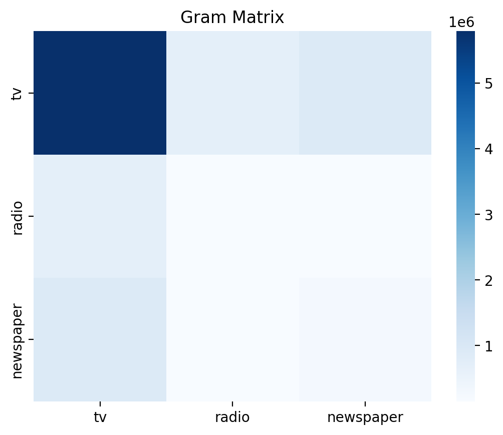
Hmm it looks like \(tv\) has a lot of variance compared to the other variables. Let’s plot them to understand what’s going on.
We’ll make a histogram of each variable just to see how spread out it is:
ax=sns.histplot(data=df, x='tv', kde=True, label='TV')
ax=sns.histplot(data=df, x='radio', kde=True, label='Radio')
ax=sns.histplot(data=df, x='newspaper', kde=True, label='Newspaper')
ax.legend();
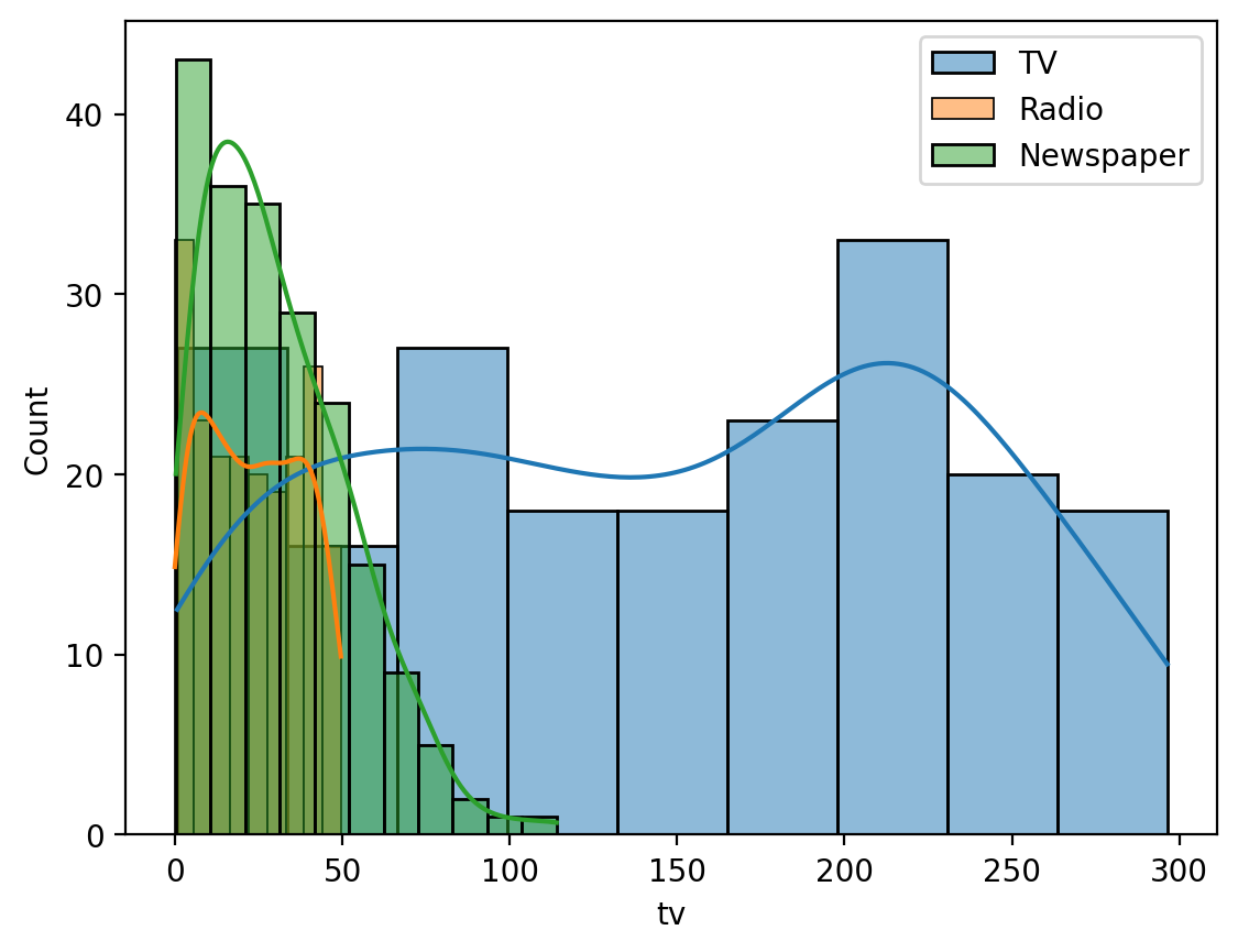
Ah we can see that \(tv\) takes on many more values than either \(radio\) or \(newspaper\) - its distribution is much wider, hence the higher value and darker color in the heatmap above. We’ll revisit this later…
Residual variance \(\sigma^2\)#
To calculate the variance of the residuals we can use the .resid attribute of the results that ols calculates for us. Since it’s a numpy array of values we can call .var() to get the variance and use ddof=4 to account for the fact that we’re estimating 4 parameters - “consuming” 4 degrees of freedom
# Variance of the residuals accounting for 4 estimated params
results.resid.var(ddof=4)
np.float64(2.8409452188887094)
It turns out that ols already calculates this for us:
# Variance of residuals that statsmodels already stores it for us
results.scale
np.float64(2.8409452188887103)
which confirms how we calculated it above. ols also stores a .mse_resid which is the mean-squared-error of the residuals.
If you remember from class: average residual variance = average model error so it should be the same value

# Remember resid variance = average error, so MSE is the same thing!
results.mse_resid
np.float64(2.8409452188887103)
Calculating SE#
Ok we have all the pieces to lets calculate the formula:
First, we calculate what it takes to “undo” the similarity between predictors using the matrix inverse:
# Calculated above
# G = X^T * X

XTXinv = np.linalg.inv(G)
Then we grab just the diagonal values - because we specifically care about the variances of each predictor not the co-variances between predictors.
diag_inv = np.diag(XTXinv)
# 4 for 4 predictors
diag_inv.shape
(4,)
Then we multiply by our average error to get the \(\text{Var}(\beta)\)
beta_var = results.mse_resid * diag_inv
And take the square root to finally get \(SE_{\hat{\beta}} = \sqrt{\text{Var}(\hat{\beta})}\)
beta_se = np.sqrt(beta_var)
beta_se
array([0.31190824, 0.0013949 , 0.00861123, 0.00587101])
In one fell-swoop this looks like:
# Altogether
np.sqrt(np.diag(results.scale * np.linalg.inv(np.dot(X.T, X)))).round(6)
array([0.311908, 0.001395, 0.008611, 0.005871])
And we can confirm against the standard-errors that ols calculated for us:
np.allclose(
    results.bse.to_numpy(),      # <- ols calculation
    beta_se                      # <- our calculation
)
True
Analytic p-value#
To make a statistical inference, we want to calculate the ratio between our signal, i.e. our estimate \(\hat{\beta}\) and our noise, i.e. our standard-error \(SE_{\hat{\beta}}\).
The larger the \(t\) the more confidence we can have in the precision of \(\hat{\beta}\).
# ols estimates
results.tvalues
Intercept     9.422288
tv           32.808624
radio        21.893496
newspaper    -0.176715
dtype: float64
# t = coef / se
np.allclose(
    results.tvalues,
    results.params / results.bse   # <- calculate them by hand
)
True
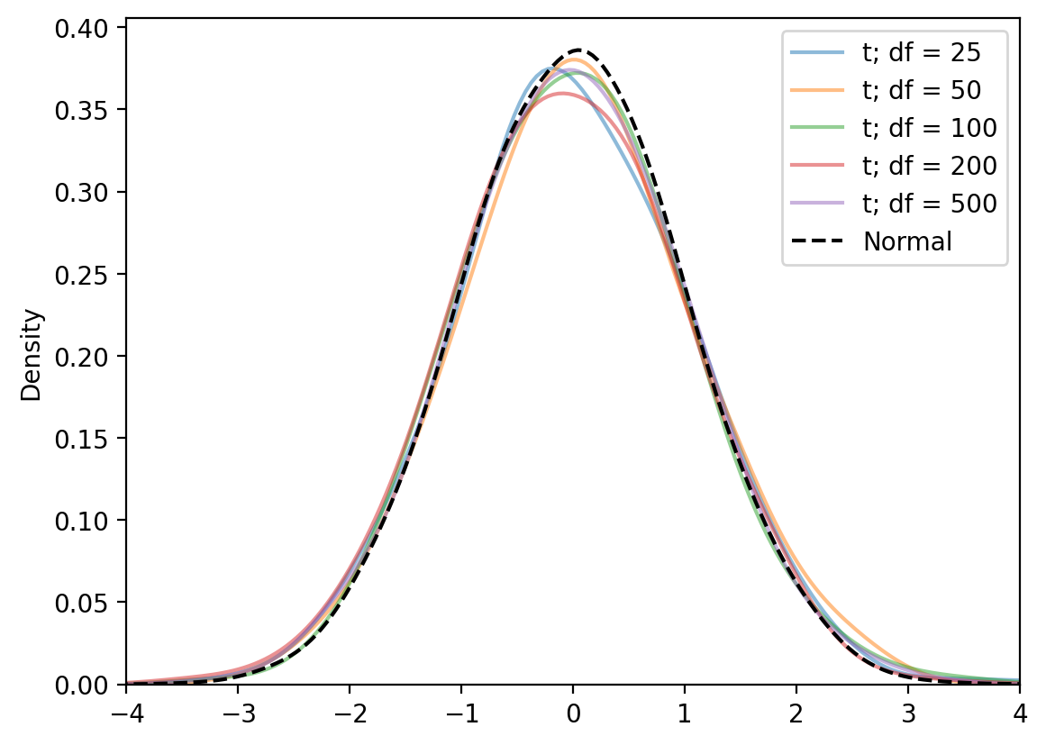
Now if we assume that the sampling distribution of this signal-to-noise-ratio \(t\) looks more and more normal as the size of our sample grows, we can use a t-distribution to look up a p-value.
Intuitively, you can think of a t-distribution as a normal distribution with fatter tails. In technical terms, it carries more probability mass in the extremes relative to a standard normal distribution. As our sample size grows, the degrees of freedom increase, and the tails thin out to look more and more normal - our t-statistic starts to look more like a z-score.
Here’s a figure demonstrating that by increasing the degrees-of-freedom of the t-distribution and comparing it to the normal distribution:
from scipy.stats import t

# Some mock sample sizes
sample_size = [25, 50, 100, 200, 500]

# KDE smoothing
bw_adjust = 1.5

# Loop over sample size and make plots
for sample in sample_size:
    data = t.rvs(df=sample,size=1000);
    sns.kdeplot(data, label=f"t; df = {sample}", alpha=.5, bw_adjust=bw_adjust);

# Add a normal distribution
ax = sns.kdeplot(np.random.normal(size=10000), label="Normal", alpha=1, color='black', bw_adjust=bw_adjust, ls='--');

# Customization
ax.set_xlim(-4,4)
plt.legend();
With this sampling distribution in hand, we can “look up” our p-value, which allows us to make the following inference:
assuming no true signal exists, how surprised we are to observe this signal-to-noise-ratio, given how many parameters we estimated overall, and the size of our sample?
In Python, we can use the cumulative distribution function of the t-distribution, to look-up the p-value using scipy like we did for the F-test previously:
# Two-sided p-value so use absolute values of t-stats
tstats = np.abs(results.tvalues.to_numpy())

# Remaining df is number of observations - number of parameters
dof = model.df_resid

# Look up the p-values using residual degrees of freedom from the model
pvals = 2 * (1 - t.cdf(tstats, df=dof))

pvals
array([0. , 0. , 0. , 0.85991505])
Which is what ols calculated for us:
np.allclose(
    pvals,
    results.pvalues.to_numpy()
)
True
Summary of parametric inference#
Parametric inference is the process of using an analytic formula to assume the shape of the sampling distribution and “look-up” a p-value
Our assumptions are only guaranteed to hold true if we have a large enough sample size
This inference process is only valid if we haven’t violated any model assumptions (e.g. no structure in our errors)
If we haven’t violated them, then the signal-to-noise ratio of an estimate \(\frac{\hat{\beta}}{SE_{\hat{\beta}}}\) will follow a t-distribution with \(n-p\) degrees of freedom
If we have, then we should not assume the shape of the sampling distribution - and either respecify our model/data or use non-parametric inference (next section)
To perform parametric inference we:
Estimate parameter \(\hat{\beta}\)
Estimate our uncertainty \(SE_{\hat{\beta}}\)
Calculate our “signal-to-noise ratio” \(t = \hat{\beta} / SE_{\hat{\beta}}\)
Look-up our p-value: assuming no true signal (i.e. \(t=0\)) what is the probability of observing a value as extreme as our \(t\)?
Non-parametric inference using bootstrap resampling#
If that was all a bit confusing or we’re not sure about violating model assumptions we can use bootstrapping to actually compute the sampling dstiributions by resampling-with-replacement from our data!

Having a large enough sample size is still important - but it makes more intuitive sense why:
If we’re building new datasets by resampling-with-replacement from our current dataset, then a smaller dataset has far few combinations of new datasets that we can generate from it! The larger our dataset, the more combinations we have to generate, which will give us a more accurate sense of the (re)-sampling distribtion that we’re building up!
Remember, what we want to know is how much \(\hat{\beta}\) will change, had we collected a different sample. So we’ll generate a new dataset, re-estimate \(\hat{\beta}\), hold on to it, create another bootstrap sample, and repeat the process. Each time \(\hat{\beta}\) will change a little bit. With enough bootstrap sample we can build-up a distribution of this variability - this is our sampling distribution - and the width of it is the uncertainty in our estimate!
Let’s write a function to do this so that we can re-use it in the future. We want our function to take in 3 arguments:
results: the output of callingmodel.fit()when we useolsnboot: the number of bootstraps to runrandom_seed: a number we can use to reproduce our random sampling
In the body of the function we want to implement a for loop logic to do the following:
Resample from
dfwith replacement using the polars.sample()methodFit a new
olsmodel to the resampled data and store it’sparams(betas)Repeat
nboottimesAt the end, use
np.stdandnp.percentileto calculate the width of this distribution and the 95% confidence intervals
Finally we’ll combine all the results into a new Dataframe called boot_results, attach it to the original results object that was input, and return it along with our boostrapped estimates:
def boot_ols(results, nboot=5000, random_seed=0):

    # A neat progress bar that replaces range()
    from tqdm import trange

    params = [] # to store the betas we estimate from each re-sampled dataset
    original_params = results.params.to_numpy() # the original betas for reference

    # For reproducibility
    np.random.seed(random_seed)

    # Start bootstrapping
    for _ in trange(nboot):

        # First generate a new dataset using the original dataframe in the results object
        # the .sample() method takes:
        # a fraction of the original data - in this case 1.0 aka 100%
        # replace - whether to sample with replacement or not
        new_data = results.model.data.frame.sample(frac=1., replace=True)

        # Fit a new regression using this data and the original model formula
        boot_model = ols(results.model.formula, new_data).fit()

        # Save the estimated betas
        params.append(boot_model.params.to_numpy())

    # Convert the list to a numpy array for convenience
    params = np.array(params)

    # Calculate the width aka the standard-deviation across bootstraps
    std_devs = np.std(params, axis=0, ddof=results.df_model)

    # Calculate the signal-to-noise aka t-statistic using the bootstrapped SD
    tstats = original_params / std_devs

    # Get the 95% CI limits using the bootstrapped estimates
    CI_limits = np.percentile(params, [2.5, 97.5], axis=0)

    # Combine into a DataFrame with original beta estimates
    boot_results = pl.DataFrame(CI_limits).transpose().with_columns(
        # Predictor names
        names = np.array(results.model.exog_names),
        # Bootstrapped SDs
        se=std_devs,
        # T-stats using boostrapped SDs
        tstats=tstats,
        # Original beta estimates
        estimate=original_params
        ).select(
            col('names').alias('variable'),
            col('estimate').alias('coef'),
            col('se').alias('boot-std'),
            col('tstats').alias('t'),
            col('column_0').alias('[0.025'),
            col('column_1').alias('0.975]'),
        )

    # Round to 5 decimal places
    boot_results = boot_results.select(
        col('variable'),
        pl.exclude("variable").round(5)
    )

    # Attach them to the result object that was passed as input
    results.boot_summary = boot_results

    # Return the results object and the bootstrapped betas
    return results, params
Let’s give our function a try by passing in the results from our estimated model
results, boot_betas = boot_ols(results, nboot=1000, random_seed=1)
100%|██████████| 1000/1000 [00:01<00:00, 572.29it/s]
We now have a new .boot_summary attribute that contains a DataFrame with the original estimates in the coef column, and boostrapped standard-deviations which were used to compute the t-statistics and confidence intervals:
results.boot_summary
| variable | coef | boot-std | t | [0.025 | 0.975] |
|---|---|---|---|---|---|
| str | f64 | f64 | f64 | f64 | f64 |
| "Intercept" | 2.93889 | 0.33699 | 8.7209 | 2.25649 | 3.57293 |
| "tv" | 0.04576 | 0.00183 | 24.98447 | 0.04215 | 0.04918 |
| "radio" | 0.18853 | 0.01104 | 17.06964 | 0.16665 | 0.20919 |
| "newspaper" | -0.00104 | 0.00675 | -0.15363 | -0.01366 | 0.01226 |
When we compare this to the analytic standard-error, t-stats, and confidence intervals from the ols model you’ll notice a few things that tend to be true in practice about bootstrapping:
t-stats will be lower
standard errors will be higher
confidence intervals will be wider
# slim=True simplifies the printed output a bit
print(results.summary(slim=True))
                            OLS Regression Results
==============================================================================
Dep. Variable:                  sales   R-squared:                       0.897
Model:                            OLS   Adj. R-squared:                  0.896
No. Observations:                 200   F-statistic:                     570.3
Covariance Type:            nonrobust   Prob (F-statistic):           1.58e-96
==============================================================================
                 coef    std err          t      P>|t|      [0.025      0.975]
------------------------------------------------------------------------------
Intercept      2.9389      0.312      9.422      0.000       2.324       3.554
tv             0.0458      0.001     32.809      0.000       0.043       0.049
radio          0.1885      0.009     21.893      0.000       0.172       0.206
newspaper     -0.0010      0.006     -0.177      0.860      -0.013       0.011
==============================================================================

Notes:
[1] Standard Errors assume that the covariance matrix of the errors is correctly specified.
This is because boostrapping allows us to make fewer assumptions about the underlying shape of the sampling distribution of our parameter estimates - we’re directly generating them.
The larger and more normally distributed your your original dataset, the less of a difference you’ll observe between bootstrapped and analytic estimates. Here’s what ours look like from the function we wrote. You’ll notice that the distributions aren’t perfectly symmetrical and have some additional density in the tails.
f, axs =plt.subplots(2,2, figsize=(10,10))
labels = ['Intercept', 'tv', 'radio', 'newspaper']

for i, ax in enumerate(axs.flat):
    _ = ax.hist(boot_betas[:,i], bins=50, color='steelblue', alpha=0.5);
    _ = ax.set_title(f"Beta_{i} = {labels[i]}");
    _ = ax.vlines(results.params.to_numpy()[i], 0, ax.get_ylim()[-1], color='black', linestyle='-');

f.suptitle("Bootstrapped Sampling Distribution of Betas", y=.95);
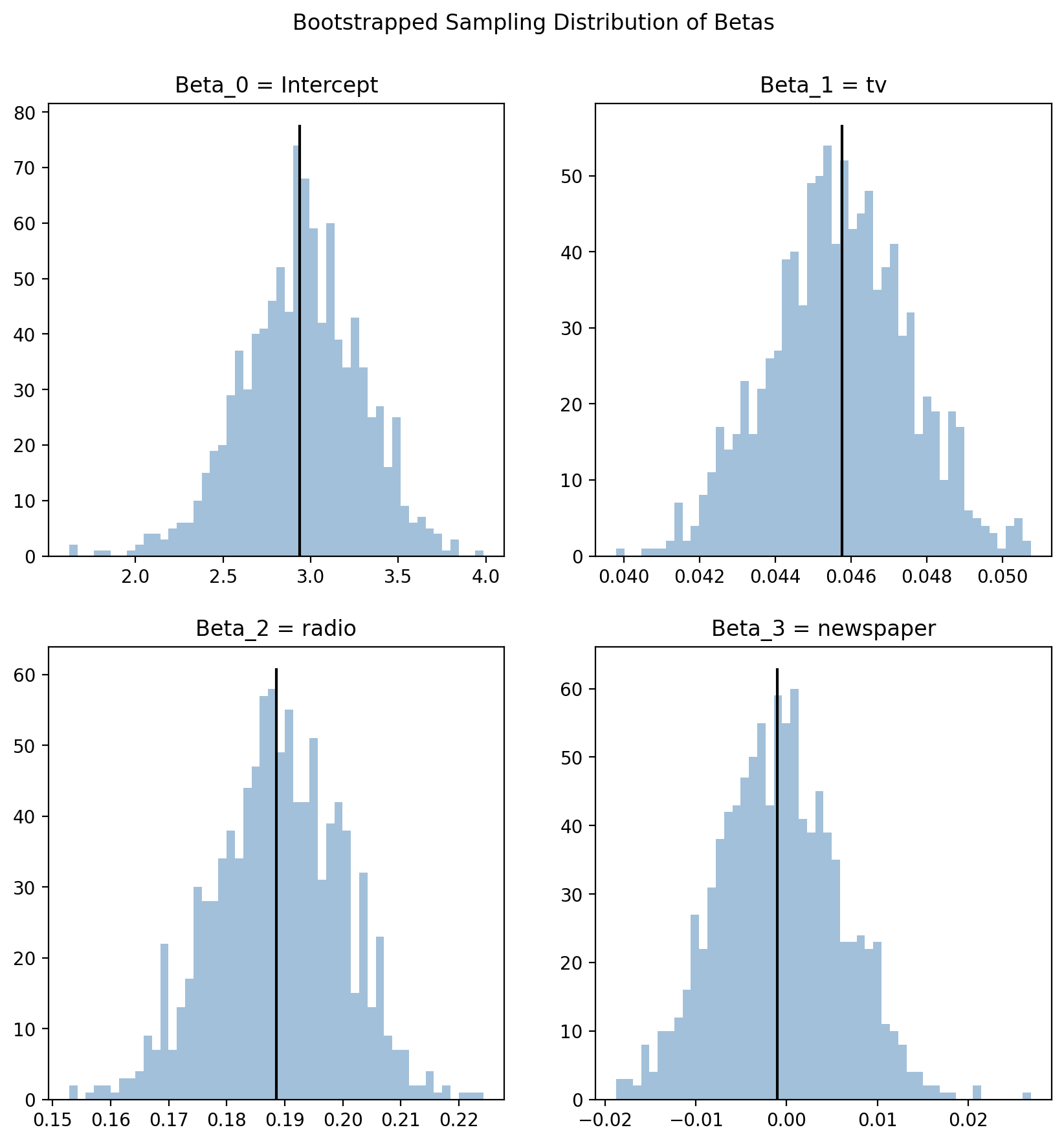
With these data, boostrapping happens to affords us the same statistical inference as the analytic approach.
For example, if we look at the predictor \(newspaper\), we see that the value \(0\) sits within the resampled distribution of estimate for \(\hat{\beta}_{newspaper}\).
And in the summary tables above, the 95% confidence intervals contain this value.
This leads us to the same inference as analytic p-value:
Factoring in the uncertainty of our estimate - the value \(0\) is not that surprising an estimate for \(\hat{\beta}_{newspaper}\) - “not statistically significant”
Non-parametric inference using permutation (shuffling)#
In addition to the uncertainty of our estimates we have one more tool to perform statistical inference: we can also use resampling to build up a null distribution.
Remember what a p-value fundamentally represents: the probability of observing our estimate like ours assuming the null hypothesis is true.
So just like we replaced our assumption about the shape of a sampling distribution with bootstrapping, we can replace our assumption about the shape of a null distribution with permutation

Let’s write another function to do this so that we can re-use it in the future. We want our function to take in 3 arguments:
results: the output of callingmodel.fit()when we useolsnperm: the number of times to shuffle the datasetrandom_seed: a number we can use to reproduce our shuffling
In the body of the function we want to implement a for loop logic to do the following:
Shuffle the rows of our dependent variable column in
dfusing the polars.sample()method which breaks its relationship to the independent variablesFit a new
olsmodel to the shuffled data and store it’stvaluesRepeat
npermtimesCalculate how often the permuted t-values were greater than our original t-value
def perm_ols(results, nperm=5000, random_seed=0):

    # A neat progress bar that replaces range()
    from tqdm import trange

    perm_ts = [] # to store the t-stats we estimate from each shuffled dataset
    original_ts = results.tvalues.to_numpy() # the original ts for reference
    dv_name = results.model.endog_names # name of y variable

    # For reproducibility
    np.random.seed(random_seed)

    for _ in trange(nperm):

        # Generate new dataset by shuffling rows in the DV column only
        # and use .alias to deliberately *overwrite* the DV column
        new_data = df.with_columns(
            df[dv_name].sample(fraction=1.,with_replacement=False,shuffle=True)
            .alias(dv_name)
            )

        # Fit model to it
        pmodel = ols(results.model.formula, data=new_data.to_pandas())
        presults = pmodel.fit()

        # Save the t-stats
        perm_ts.append(presults.tvalues.to_numpy())

    perm_ts = np.array(perm_ts)

    # Get the # of permuted t-stats >= observed t-stat
    proportion = np.sum(
        np.abs(perm_ts) >= np.abs(original_ts),
        axis=0) + 1

    # Divide by number of permutation to get p-value
    # Add 1 to numerator and denominator to avoid divide-by-zero errors
    pvals = proportion / (nperm + 1)

    # Make a polars DataFrame
    pvals = pl.DataFrame(dict(zip(results.model.exog_names, pvals)))

    # Shuffling the data doesn't permute the intercept so ignore the p-value
    pvals[0, 'Intercept'] = np.nan

    # Return pvals and permuted t-stats
    return pvals, perm_ts
And trying it out we can see our permuted p-values are very similar to the analytic p-values from ols:
pvals, perm_ts = perm_ols(results, nperm=1000, random_seed=1)
100%|██████████| 1000/1000 [00:01<00:00, 523.23it/s]
pvals
| Intercept | tv | radio | newspaper |
|---|---|---|---|
| f64 | f64 | f64 | f64 |
| NaN | 0.000999 | 0.000999 | 0.861139 |
# From ols
results.pvalues.round(5)
Intercept    0.00000
tv           0.00000
radio        0.00000
newspaper    0.85992
dtype: float64
And we can visualize our null distributions which show us what t-statistics we would expect under the assumption that there is no relationship between our \(y\) (\(sales\)) and our \(X\) (\(tv\), \(radio\), \(newspaper\)) variables.
We simulated this assumption by randomizing our data via shuffling (permutation).
f, axs =plt.subplots(3,1, figsize=(10,10), sharey=False, sharex=False)
labels = ['tv', 'radio', 'newspaper']

for i, ax in enumerate(axs.flat):
    _ = ax.hist(perm_ts[:,i+1], bins=50, color='steelblue', alpha=0.5);
    _ = ax.set_title(f"Null for {labels[i]}");
    _ = ax.set_ylabel("Count");
    _ = ax.vlines(results.tvalues.to_numpy()[i+1], 0, ax.get_ylim()[-1], color='black', linestyle='-');

f.suptitle("Permuted Null Distribution of T-stats", y=.95);
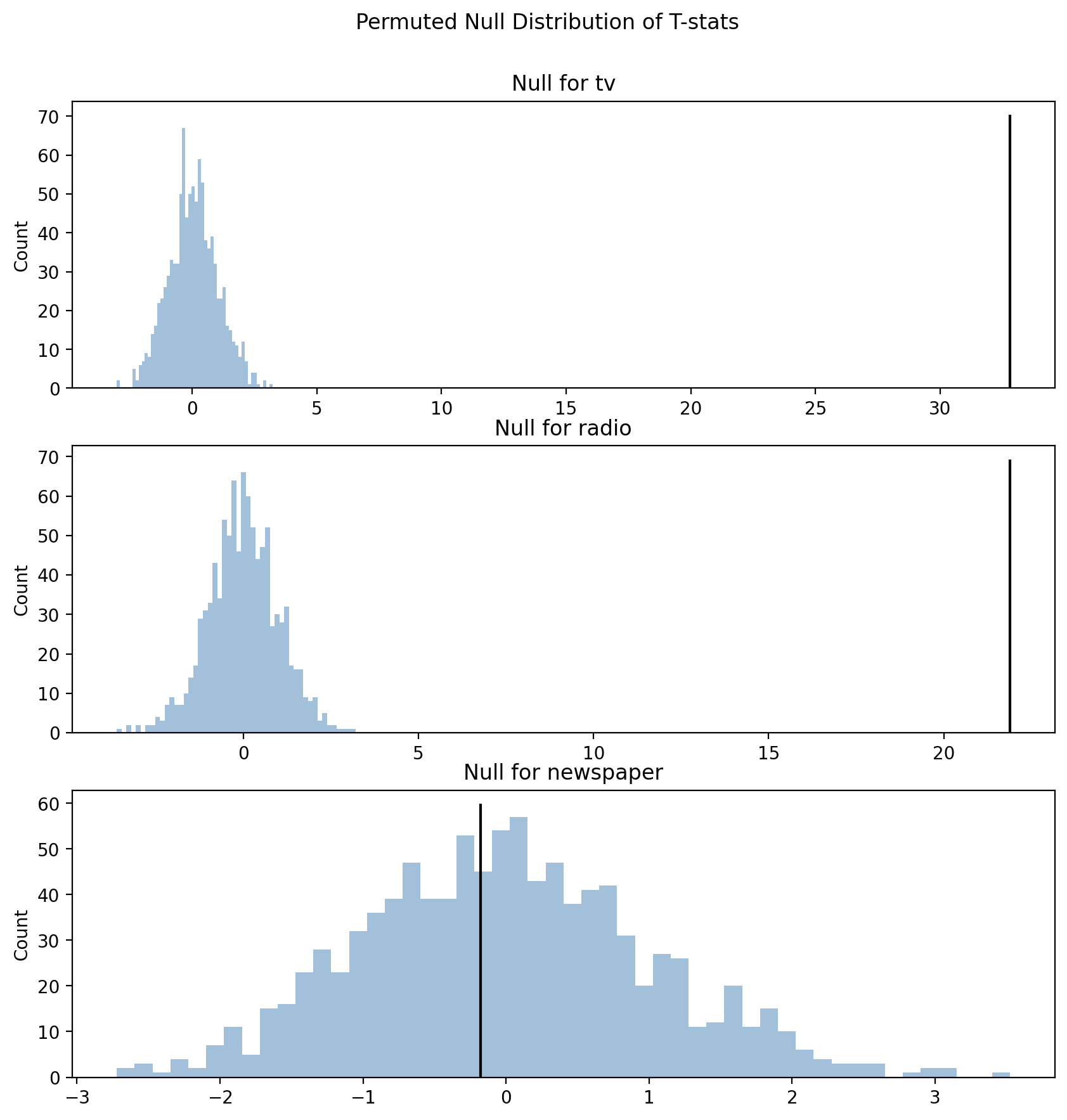
It’s very clear from these plots why \(newspaper\) (bottom) is not “statistically significant” -
the signal-to-noise ratio \(t\) is well-within the range of values we would expect assuming our data were random!
Summary of non-parametric inference via permutation#
Permutation allows us to build null distributions to perform statistical inference on our parameter estimates
Based on how we choose randomize we can simulate the specific form of randomization that we what to make an inference about
In the example above we preserved the relationship between the predictors, by only permuting the response variable
To perform a permutation test with a GLM we can:
Fit our model and calculate our inferential statistic - the one we want a p-value for \(t\)
Shuffle our response variable \(y\) and re-estimate our model using the shuffled data
Repeat this process with more randomizations
Calculate the proportion of times the permuted versions of our inferential statistic \(t\) are greater-than-or-equal-to our observed value \(t\) on the original data
Challenge Q (response)#
What do you think would happen if you instead shuffled a column of one of the predictor variables?
Your response here
General summary of Non-Parametric Inference#
With these two approach to resampling we can make fewer assumptions about the structure of our model’s errors and just calculate them directly from our data. The biggest trade-off to these approaches is that they are more “expensive” to calculate - but when possible - especially with complicated datasets - they often yield more robust and verifiable inferences; when in doubt - just inspect the resampling or null distributions you created!
Regardless of whether you use parametric or non-parametric inference it’s important to understand why statistical signficance IS NOT practical or scientific significance.
The standard-error and ultimately the t-stat and p-value reflect a combination of the following:
size of the \(\beta\)
how bad the model is overall
the sample size
the variance of the \(Xn\) that \(\beta\) corresponds to
and the correlation of \(Xn\) with all other columns in \(X\)
To paraphrase from one of the assigned readings, The Truth About Linear Regression:
This means that the standard errors will shrink as the sample size grows, so more and more variables will become significant as we get more data — but how much data we collect is irrelevant to how the process we’re studying actually works! Moreover, at a fixed sample size, the coefficients with smaller standard errors will tend to be the ones whose variables have more variance, and whose variables are less correlated with the other predictors. High input variance and low correlation help us estimate the coefficient precisely, but, again, they have nothing to do with whether the input variable actually influences the response a lot!
To sum up, it is never the case that statistical significance is the same as scientific, real-world significance. The most important variables are not those with the largest-magnitude t statistics or smallest p-values. Statistical significance is always about what “signals” can be picked out clearly from background noise. In the case of linear regression coefficients, statistical significance runs together the size of the coefficients, how bad the linear regression model is, the sample size, the variance in the input variable, and the correlation of that variable with all the others. Of course, even the limited “does it help linear predictions enough to bother with?” utility of the usual t-test (and F-test) calculations goes away if the standard distributional assumptions do not hold, so that the calculated p-values are just wrong. But one can sometimes get away with using bootstrapping (Chapter 6) to get accurate p-values for standard tests under non-standard conditions
Paul Meehl noted the same dilemma if we use parametric inference as our only tool to perform Null-Hypothesis-Significance-Testing (NHST):
In the limit of an infinitely large sample size, we have the least uncertainty (highest precision) to estimate a parameter. But counter-intuitively, that means that any non-zero estimate, no matter how small will appear “statistically significant” from 0 even if it’s not practically meaningful!
Wrap-up#
Let’s wrap-up by writing a convenience function that “wraps” the 2 functions we wrote above. This will make it make this even easier to use we can tweak it so it feels like a drop-in replacement for ols:
We’ll copy the definitions of our 2 function above inside the body of our new function and add a little bit of code to combine the outputs:
def ols_nonparam(formula, data, nsim=1000, random_seed=None, return_dists=False):
    """
    Non-parametric version of statsmodels OLS regression.
    Is equivalent to the output of ols(formula).fit() - in other words only returns
    the results not the model itself. The results also includes a .summary_resampled
    attribute that contains the bootstrapped and permuted results.

    Args:
        formula (str): formula to fit model
        data (DataFrame): pandas or polars DataFrame
        nsim (int, optional): number of bootstraps and permutations to run. Defaults to 1000.
        random_seed (int, optional): for reproducibility. Defaults to None.
        return_dists (bool, optional): whether to return the bootstrapped and permuted results. Defaults to False.

    Returns:
        results: statsmodels OLS regression results
    """

    from statsmodels.formula.api import ols

    # Create and fit the original model on the original data
    model = ols(formula, data)
    results = model.fit()

    # Define bootstrap function
    def boot_ols(results, nboot, random_seed):

        # A neat progress bar that replaces range()
        from tqdm import trange

        params = [] # to store the betas we estimate from each re-sampled dataset
        original_params = results.params.to_numpy() # the original betas for reference

        # For reproducibility
        np.random.seed(random_seed)

        # Start bootstrapping
        for _ in trange(nboot):

            # Resample with replacement - using pandas here instead of polars
            new_data = results.model.data.frame.sample(frac=1., replace=True)

            # Fit a new regression using this data and the original model formula
            boot_model = ols(results.model.formula, new_data).fit()

            # Save the estimated betas
            params.append(boot_model.params.to_numpy())

        # Convert the list to a numpy array for convenience
        params = np.array(params)

        # Calculate the width aka the standard-deviation across bootstraps
        std_devs = np.std(params, axis=0, ddof=results.df_model)

        # Calculate the signal-to-noise aka t-statistic using the bootstrapped SD
        tstats = original_params / std_devs

        # Get the 95% CI limits using the bootstrapped estimates
        CI_limits = np.percentile(params, [2.5, 97.5], axis=0)

        # Combine into a DataFrame with original beta estimates
        boot_results = pl.DataFrame(CI_limits).transpose().with_columns(
            # Predictor names
            names = np.array(results.model.exog_names),
            # Bootstrapped SDs
            se=std_devs,
            # T-stats using boostrapped SDs
            tstats=tstats,
            # Original beta estimates
            estimate=original_params
            ).select(
                col('names').alias('variable'),
                col('estimate').alias('coef'),
                col('se').alias('boot-std'),
                col('tstats').alias('t'),
                col('column_0').alias('[0.025'),
                col('column_1').alias('0.975]'),
            )

        # Round to 5 decimal places
        boot_results = boot_results.select(
            col('variable'),
            pl.exclude("variable").round(5)
        )

        return boot_results, params

    # Define permutation function
    def perm_ols(results, nperm, random_seed):

        # A neat progress bar that replaces range()
        from tqdm import trange

        perm_ts = [] # to store the t-stats we estimate from each shuffled dataset
        original_ts = results.tvalues.to_numpy() # the original ts for reference
        dv_name = results.model.endog_names # name of y variable

        # For reproducibility
        np.random.seed(random_seed)

        for _ in trange(nperm):

            # Convert to polars for easier shuffling
            new_data = pl.DataFrame(data)
            new_data = new_data.with_columns(
                new_data[dv_name].sample(fraction=1.,with_replacement=False,shuffle=True)
                .alias(dv_name)
                )

            # Fit model to it; and convert back to pandas
            pmodel = ols(results.model.formula, data=new_data.to_pandas())
            presults = pmodel.fit()

            # Save the t-stats
            perm_ts.append(presults.tvalues.to_numpy())

        perm_ts = np.array(perm_ts)

        # Get the # of permuted t-stats >= observed t-stat
        proportion = np.sum(
            np.abs(perm_ts) >= np.abs(original_ts),
            axis=0) + 1

        # Divide by number of permutation to get p-value
        # Add 1 to numerator and denominator to avoid divide-by-zero errors
        pvals = proportion / (nperm + 1)

        # Make a polars DataFrame
        pvals = pl.DataFrame(dict(zip(results.model.exog_names, pvals)))

        # Shuffling the data doesn't permute the intercept so ignore the p-value
        pvals[0, 'Intercept'] = np.nan

        # Return pvals and permuted t-stats
        return pvals, perm_ts

    # Run boostrapping and permuting
    boot_results, boot_betas = boot_ols(results, nsim, random_seed)
    pvals, perm_ts = perm_ols(results, nsim, random_seed)

    # Combine bootstrapped and permutation estimates into 1 DataFrame
    full_results = boot_results.with_columns(
        perm_p = pvals.to_numpy().flatten()

    )

    # Reorder columns to match ols output
    full_results = full_results.select(
        col('variable'),
        col('coef'),
        col('boot-std'),
        col('t'),
        col('perm_p').alias('P_perm>|t|'),
        col('[0.025'),
        col('0.975]')
    )

    # Attach to results object from ols
    results.summary_resampled = full_results

    # Return distributions of boostraps and permutation if requested
    if return_dists:
        return results, boot_betas, perm_ts
    else:
        return results
Let’s try our function out! We can check-out the help we wrote:
ols_nonparam?
Signature:
ols_nonparam(
    formula,
    data,
    nsim=1000,
    random_seed=None,
    return_dists=False,
)
Docstring:
Non-parametric version of statsmodels OLS regression.
Is equivalent to the output of ols(formula).fit() - in other words only returns
the results not the model itself. The results also includes a .summary_resampled
attribute that contains the bootstrapped and permuted results.

Args:
    formula (str): formula to fit model
    data (DataFrame): pandas or polars DataFrame
    nsim (int, optional): number of bootstraps and permutations to run. Defaults to 1000.
    random_seed (int, optional): for reproducibility. Defaults to None.
    return_dists (bool, optional): whether to return the bootstrapped and permuted results. Defaults to False.

Returns:
    results: statsmodels OLS regression results
File:      /var/folders/4y/y26_jdm57m90f4s1td24ls040000gn/T/ipykernel_33472/992760803.py
Type:      function
And run it on our data:
results = ols_nonparam("sales ~ tv + radio + newspaper", data=df.to_pandas(), nsim=1000, random_seed=1)
100%|██████████| 1000/1000 [00:01<00:00, 577.77it/s]
100%|██████████| 1000/1000 [00:01<00:00, 531.94it/s]
We can access the non-parametric results via the .summary_resampled attribute of the output:
results.summary_resampled
| variable | coef | boot-std | t | P_perm>|t| | [0.025 | 0.975] |
|---|---|---|---|---|---|---|
| str | f64 | f64 | f64 | f64 | f64 | f64 |
| "Intercept" | 2.93889 | 0.33699 | 8.7209 | NaN | 2.25649 | 3.57293 |
| "tv" | 0.04576 | 0.00183 | 24.98447 | 0.000999 | 0.04215 | 0.04918 |
| "radio" | 0.18853 | 0.01104 | 17.06964 | 0.000999 | 0.16665 | 0.20919 |
| "newspaper" | -0.00104 | 0.00675 | -0.15363 | 0.87013 | -0.01366 | 0.01226 |
And compare them to the parametric results that ols calculates for us:
results.summary(slim=True)
| Dep. Variable: | sales | R-squared: | 0.897 |
|---|---|---|---|
| Model: | OLS | Adj. R-squared: | 0.896 |
| No. Observations: | 200 | F-statistic: | 570.3 |
| Covariance Type: | nonrobust | Prob (F-statistic): | 1.58e-96 |
| coef | std err | t | P>|t| | [0.025 | 0.975] | |
|---|---|---|---|---|---|---|
| Intercept | 2.9389 | 0.312 | 9.422 | 0.000 | 2.324 | 3.554 |
| tv | 0.0458 | 0.001 | 32.809 | 0.000 | 0.043 | 0.049 |
| radio | 0.1885 | 0.009 | 21.893 | 0.000 | 0.172 | 0.206 |
| newspaper | -0.0010 | 0.006 | -0.177 | 0.860 | -0.013 | 0.011 |
Notes:
[1] Standard Errors assume that the covariance matrix of the errors is correctly specified.
Now we have a quick way to checkout our non-parametric estimates alongside our parametric ones! For future assignments we’ll try to include this function in a file that you can import. But it might be handy to refer to this notebook if you ever need to write it again.
Challege: Non-Parametric Inference#
Below we’ve loaded up Anscombe’s Quartet again and plotted a simple univariate regression using sns.lmplot, which uses ols behind-the-scenes.
When you run the cell you’ll see the regression line for each dataset and 95% bootstrapped confidence intervals that seaborn automatically computed for us.
# Load and convert to polars
anscombe = pl.DataFrame(sns.load_dataset("anscombe"))

# Plot the regression for each dataset separately
sns.lmplot(x="x", y="y", data=anscombe, hue="dataset", col='dataset', col_wrap=2, height=2)
<seaborn.axisgrid.FacetGrid at 0x16c8af8d0>
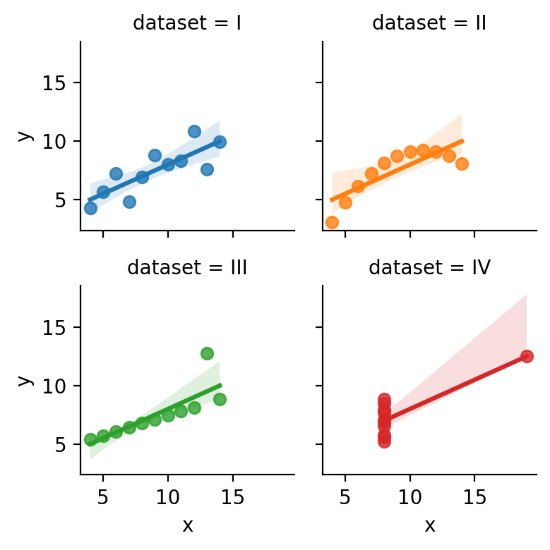
Looking at each sub-plot above, it seems like the the “worst” fit is with dataset IV.
In every other dataset there seems to be some type of relationship between x and y - but in dataset IV this seems to be driven by a single observation.
Your task is to fit a univariate regression to dataset IV only using the new ols_nonparam function we wrote.
You’ll have to use .filter() to subset the rows in anscombe that you want.
For ols_nonparam you can use:
nsim=2000random_seed=1return_dists=True
# Solution
data_4 = anscombe.filter(col("dataset") == "IV")
# Solution
results, boots, perms = ols_nonparam('y ~ x', data=data_4.to_pandas(), nsim=2000,random_seed=1, return_dists=True)
100%|██████████| 2000/2000 [00:02<00:00, 846.91it/s]
100%|██████████| 2000/2000 [00:03<00:00, 617.38it/s]
Inspect the differences in the outputs of .summary_resampled and .summary()
What do you notice?
# Solution
results.summary_resampled
results.summary(slim=True)
| variable | coef | boot-std | t | P_perm>|t| | [0.025 | 0.975] |
|---|---|---|---|---|---|---|
| str | f64 | f64 | f64 | f64 | f64 | f64 |
| "Intercept" | 3.00173 | 1.48395 | 2.02279 | NaN | 0.10001 | 4.12477 |
| "x" | 0.49991 | 0.17794 | 2.80946 | 0.064468 | 0.4408 | 0.92688 |
/Users/esh/miniconda3/envs/201b/lib/python3.11/site-packages/scipy/stats/_axis_nan_policy.py:418: UserWarning: `kurtosistest` p-value may be inaccurate with fewer than 20 observations; only n=11 observations were given.
  return hypotest_fun_in(*args, **kwds)
| Dep. Variable: | y | R-squared: | 0.667 |
|---|---|---|---|
| Model: | OLS | Adj. R-squared: | 0.630 |
| No. Observations: | 11 | F-statistic: | 18.00 |
| Covariance Type: | nonrobust | Prob (F-statistic): | 0.00216 |
| coef | std err | t | P>|t| | [0.025 | 0.975] | |
|---|---|---|---|---|---|---|
| Intercept | 3.0017 | 1.124 | 2.671 | 0.026 | 0.459 | 5.544 |
| x | 0.4999 | 0.118 | 4.243 | 0.002 | 0.233 | 0.766 |
Notes:
[1] Standard Errors assume that the covariance matrix of the errors is correctly specified.
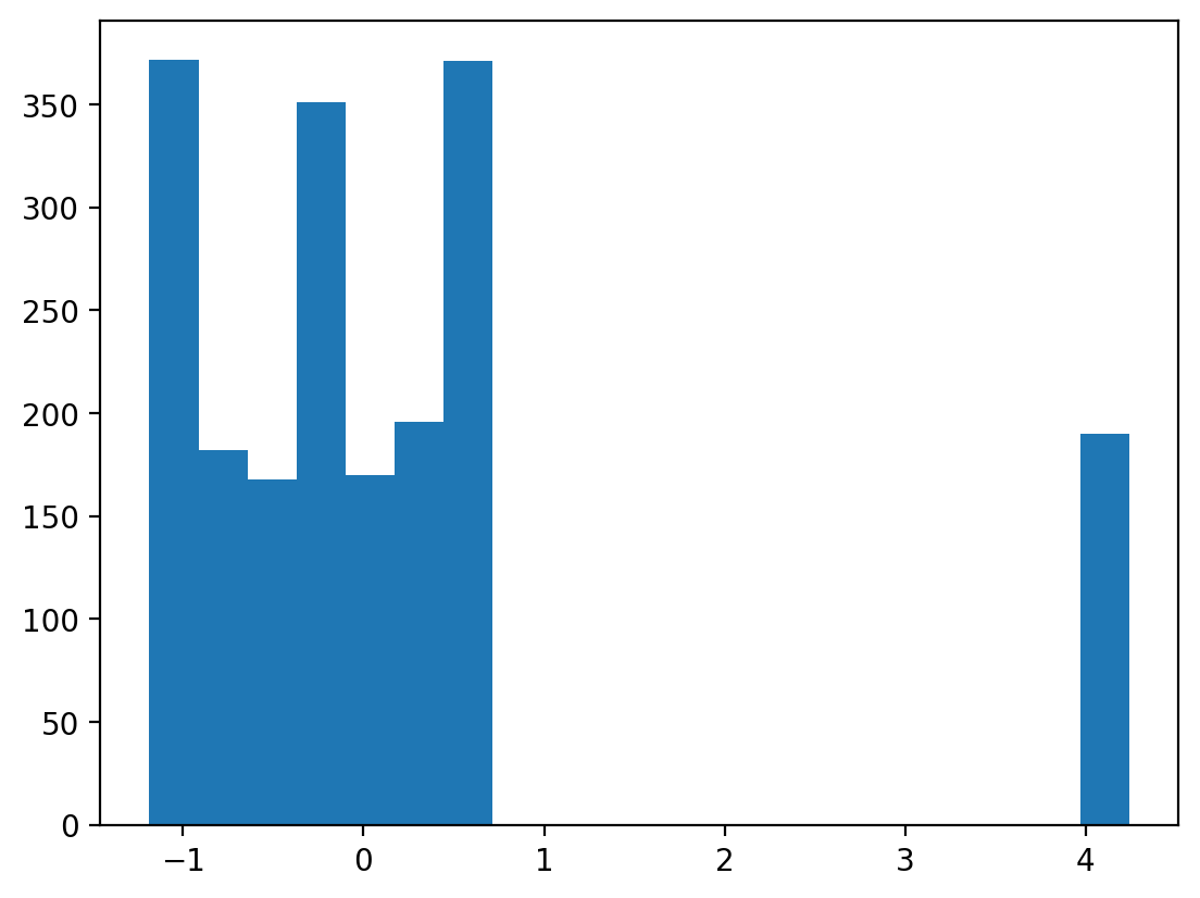
Inspect perms using a histogram.
You can use perms = perm[:, 1] before plotting to only plot the permuted values for x and ignore the model intercept
What do you notice? How does this affect the permuted p-value vs the analytic p-value in the outputs above?
# Solution
# Ignore intercept
perms = perms[:, 1]
plt.hist(perms, bins=20)
(array([372., 182., 168., 351., 170., 196., 371.,   0.,   0.,   0.,   0.,
          0.,   0.,   0.,   0.,   0.,   0.,   0.,   0., 190.]),
 array([-1.18601317, -0.9145611 , -0.64310903, -0.37165696, -0.1002049 ,
         0.17124717,  0.44269924,  0.71415131,  0.98560337,  1.25705544,
         1.52850751,  1.79995958,  2.07141165,  2.34286371,  2.61431578,
         2.88576785,  3.15721992,  3.42867199,  3.70012405,  3.97157612,
         4.24302819]),
 <BarContainer object of 20 artists>)