Models VII: 3+ level categorical predictors & One-way ANOVA#
In notebook 05_models we saw how we can encode a categorical predictor with 2-levels (Student = (Yes or No)) in a GLM using treatment (dummy) codes.
Let’s extend this idea to explore how to model categorical variables with more thant 2 levels
We’re going to look at a new dataset that comes from the following paper:
The experiments used a 2 (skill) x 3 (hand) x 2 (limit) design
This is reflected in the provided tidy-dataset which has 4 columns:
Variable |
Description |
|---|---|
skill |
a player’s skill (expert/average) |
hand |
the quality of the hand experimenters manipulate (bad/neutral/good) |
limit |
the style of game (fixed/no-limit) |
balance |
a player’s final balance in Euros |
Slides for reference#
Data#
Let’s load the data and verify the details above:
import numpy as np
import polars as pl
from polars import col
import seaborn as sns
import matplotlib.pyplot as plt
from statsmodels.formula.api import ols
from statsmodels.stats.anova import anova_lm
df = pl.read_csv('./data/poker-tidy.csv')
df.head()
| skill | hand | limit | balance |
|---|---|---|---|
| str | str | str | f64 |
| "expert" | "bad" | "fixed" | 4.0 |
| "expert" | "bad" | "fixed" | 5.55 |
| "expert" | "bad" | "fixed" | 9.45 |
| "expert" | "bad" | "fixed" | 7.19 |
| "expert" | "bad" | "fixed" | 5.71 |
This reflects the 300 participants in the experiment and 4 columns of our dataframe:
df.shape
(300, 4)
Challenge: Using polars, figure out how many observations there are per cell of the 2x3x2 design
# Your code here
# Solution
df.group_by(['skill','hand', 'limit']).len()
| skill | hand | limit | len |
|---|---|---|---|
| str | str | str | u32 |
| "expert" | "neutral" | "fixed" | 25 |
| "average" | "neutral" | "no-limit" | 25 |
| "average" | "good" | "fixed" | 25 |
| "expert" | "bad" | "fixed" | 25 |
| "expert" | "good" | "no-limit" | 25 |
| … | … | … | … |
| "average" | "good" | "no-limit" | 25 |
| "average" | "bad" | "fixed" | 25 |
| "average" | "bad" | "no-limit" | 25 |
| "expert" | "neutral" | "no-limit" | 25 |
| "expert" | "good" | "fixed" | 25 |
Categorical Predictor with 3 levels#
The first question we’re interested in testing is: does having a better hand earn more money, i.e a higher balance?
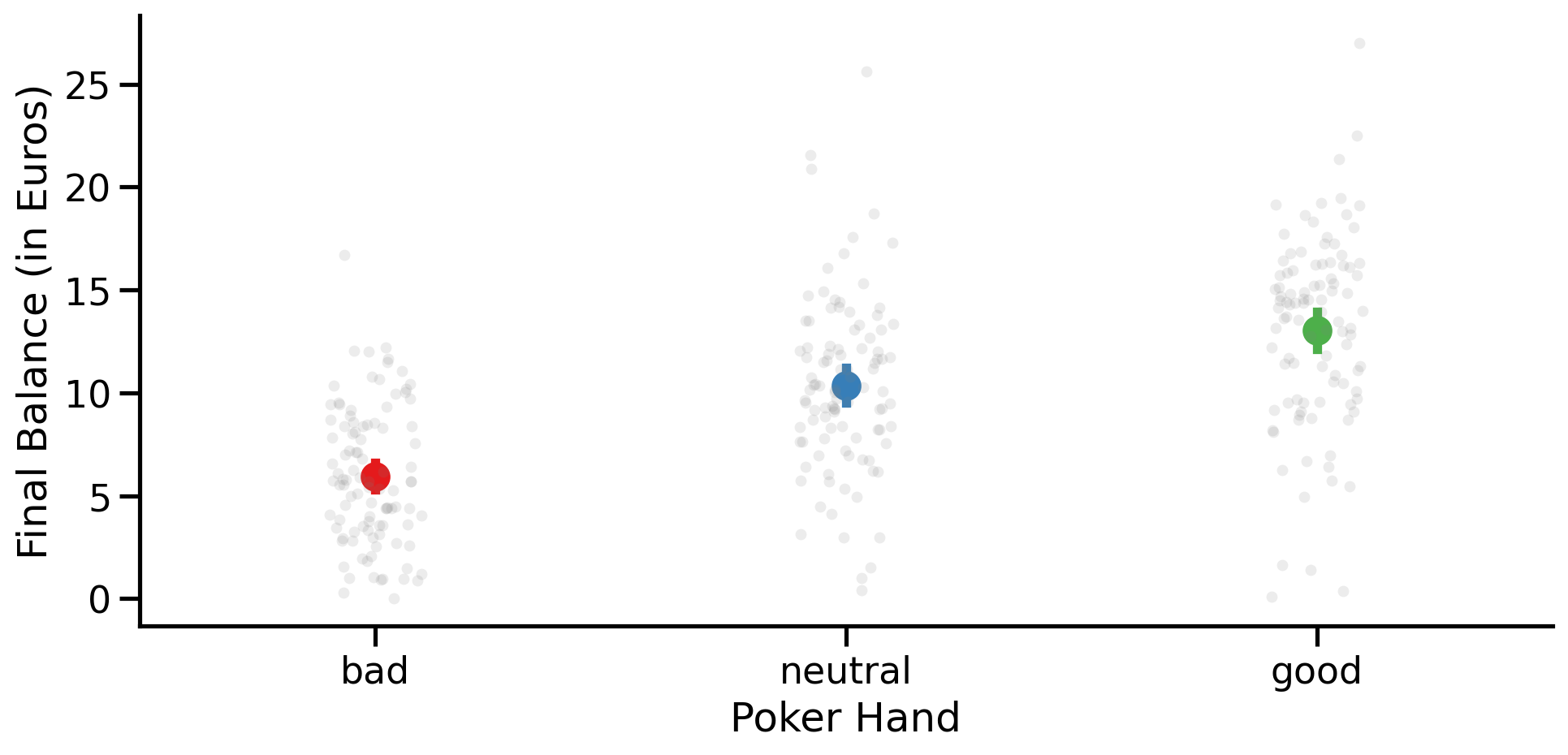
Challenge: Visualization#
Create a figure that plots data from each level of hand on the x-axis and balance on the y-axis
Add a bar or point that also reflect the mean balance at each level
# Your code here
# Solution
order = ['bad', 'neutral', 'good']
with sns.plotting_context('talk'):
    grid = sns.FacetGrid(data=df, height=5, aspect=2)
    grid = grid.map(sns.stripplot, 'hand', 'balance', order=order, alpha=0.15, color='gray')
    grid.map_dataframe(sns.pointplot, 'hand', 'balance', hue='hand', order=order, hue_order=order, palette='Set1')
    grid.set_axis_labels('Poker Hand', 'Final Balance (in Euros)');
<seaborn.axisgrid.FacetGrid at 0x10df0ddd0>
<seaborn.axisgrid.FacetGrid at 0x10df0ddd0>
Challenge: Worth it?#
Like previous notebooks start by defining a compact model and an augmented model and then comparing them to see whether adding hand to a model reduces enough error to be worth it:
# Your code here
# Solution
# Compact
model_c = ols('balance ~ 1', data=df.to_pandas())
results_c = model_c.fit()

# Augmented
model_a = ols('balance ~ C(hand)', data=df.to_pandas())
results_a = model_a.fit()

# Worth it?
anova_lm(results_c, results_a)
| df_resid | ssr | df_diff | ss_diff | F | Pr(>F) | |
|---|---|---|---|---|---|---|
| 0 | 299.0 | 7579.984625 | 0.0 | NaN | NaN | NaN |
| 1 | 297.0 | 5020.583223 | 2.0 | 2559.401402 | 75.702581 | 2.699281e-27 |
Use anova_lm with just your augmented model and the argument type=3 to generate a One-way ANOVA table. How does this compare to model comparison you just did?
# Solution
anova_lm(results_a, type=3)
| df | sum_sq | mean_sq | F | PR(>F) | |
|---|---|---|---|---|---|
| C(hand) | 2.0 | 2559.401402 | 1279.700701 | 75.702581 | 2.699281e-27 |
| Residual | 297.0 | 5020.583223 | 16.904321 | NaN | NaN |
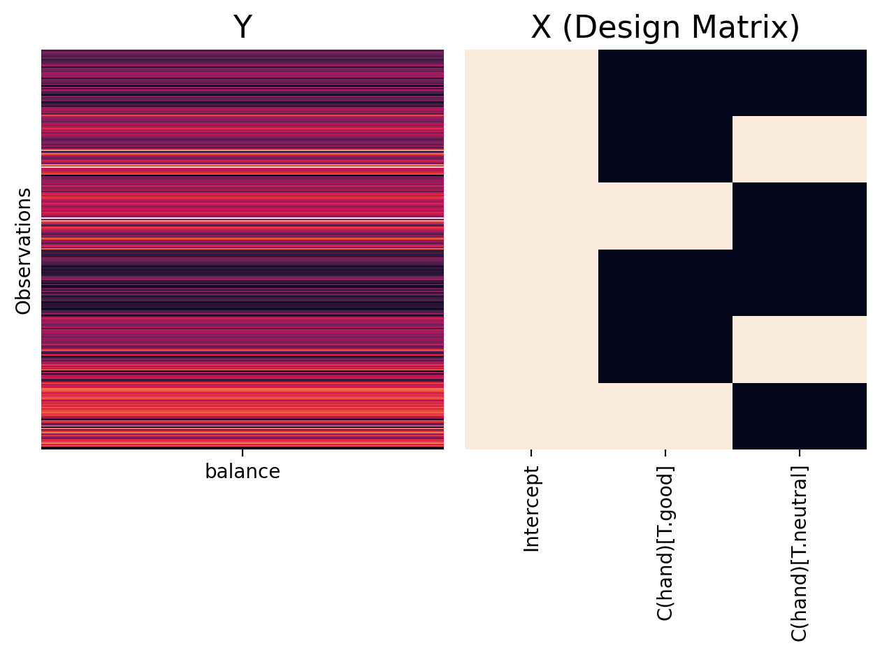
Interpreting Parameters#
Let’s try to understand how the GLM represented the levels of hand
Remember that the default for C() is to represent our categorical variable using treatment/dummy codes - with the reference level being the alphabetically first level in the data.
Using our helper plottign function we can visualize the design matrix for our model and see that it created 2 additional columns to represent hand. In this case:
Intercept = mean of
hand = 'bad'\(\beta_1\) = difference between
hand = 'good'andhand = 'bad'\(\beta_2\) = difference between
hand = 'neutral'andhand = 'bad'
from helpers import plot_design_matrix

# In case you named your model something different above we redefine it here
model_a = ols('balance ~ C(hand)', data=df.to_pandas())

plot_design_matrix(model_a)
Challenge#
Use polars to calculate the mean for each level of hand. Then using the explanation of dummy-coding above, use the means to recreate what each parameter estimate represents.
Use print in Python or a markdown cell to write out your explanation
# Here are the parameters
# Can you get these values by using the means of each level of hand?
results_a.params
Intercept             5.9415
C(hand)[T.good]       7.0849
C(hand)[T.neutral]    4.4051
dtype: float64
# Your code here
# Solution
hand_means = df.group_by('hand', maintain_order=True).agg(col('balance').mean())
bad = hand_means[0,1]
neutral = hand_means[1,1]
good = hand_means[2,1]

print(f'Intercept = Bad hand: {bad:.3f}')
print(f"B1 = Good - Bad: {good - bad:.3f}")
print(f"B2 = Neutral - Bad: {neutral - bad:.3f}")
Intercept = Bad hand: 5.941
B1 = Good - Bad: 7.085
B2 = Neutral - Bad: 4.405
Additional Coding Systems for Categorical Variables#
What if we want to represent the levels of our categorical variable in different way? We already saw how to change the reference level when using treatment/dummy codes - but we can also use an entirely different approach.
In this section we’ll cover the 2 additional common ways to encode categorical variables:
Deviation (Sum) Coding
Orthogonal Polynomial Coding
The reason to understand these additional encoding schemes is that they provide valid inferences when we extend our model to include additional categorical or continuous predictors.
Below we provide a brief overview of each coding scheme and how to use it but you should check-out the following resources as part of this lab as well:
Coding Systems for Categorical Variables conceptual overview, but examples are in R
Contrasts in StatsModels Shorter Python version of the guide above
Scheme Name |
Intercept Interpretation |
Other Parameters Interpretation |
Formula Syntax |
Affected by Unbalanced Designs? |
Typical Usage |
Additional Notes or Customizations |
Interpretation Warnings and Guidance |
|---|---|---|---|---|---|---|---|
Treatment (Dummy) |
Baseline (reference) category |
Difference from the reference category |
|
Yes |
Default; good for categorical predictors with a natural reference |
Reference level can be set via |
Be mindful of choosing a meaningful reference category |
Deviation (Sum) |
Grand mean |
Difference from grand mean |
|
No |
ANOVA-style contrasts; balanced designs |
Ensures sum of contrasts = 0 |
In unbalanced designs, parameter estimates may not match simple group means |
Polynomial |
Linear trend |
Higher-order polynomial trends |
|
No |
Modeling trends in ordered categories |
Useful for variables with lots of levels |
|
Deviation (Sum/Contrast) Coding#
This form of coding uses the intercept to estimate the grand-mean (mean of means) of all levels and uses additional parameters to calculate the difference between each level and the grand-mean. This coding scheme is very useful when we have categorical variables with 3+ levels and uneven group sizes and want to perform valid F-tests (ANOVAs).
In the case of 2-levels \(\hat{\beta_1}\) = 2x mean difference between levels
We can use this coding scheme with C(hand, Sum)
We will have 2 columns in our design matrix but now they encode good and neutral using 1s and 0s and represent bad using -1s.
# Estimate model
model_sum = ols("balance ~ C(hand, Sum(omit='bad'))", data=df.to_pandas())
results_sum = model_sum.fit()
# Print first 10 rows of the design matrix
model_sum.exog[:10, :]
array([[ 1., -1., -1.],
       [ 1., -1., -1.],
       [ 1., -1., -1.],
       [ 1., -1., -1.],
       [ 1., -1., -1.],
       [ 1., -1., -1.],
       [ 1., -1., -1.],
       [ 1., -1., -1.],
       [ 1., -1., -1.],
       [ 1., -1., -1.]])
# Visualize the design matrix, adjust names, and add colorbar
plot_design_matrix(model_sum,
                    plot_names=['Intercept', 'C(hand, Sum)[S.good]', 'C(hand, Sum)[S.neutral]'], cbar=True)
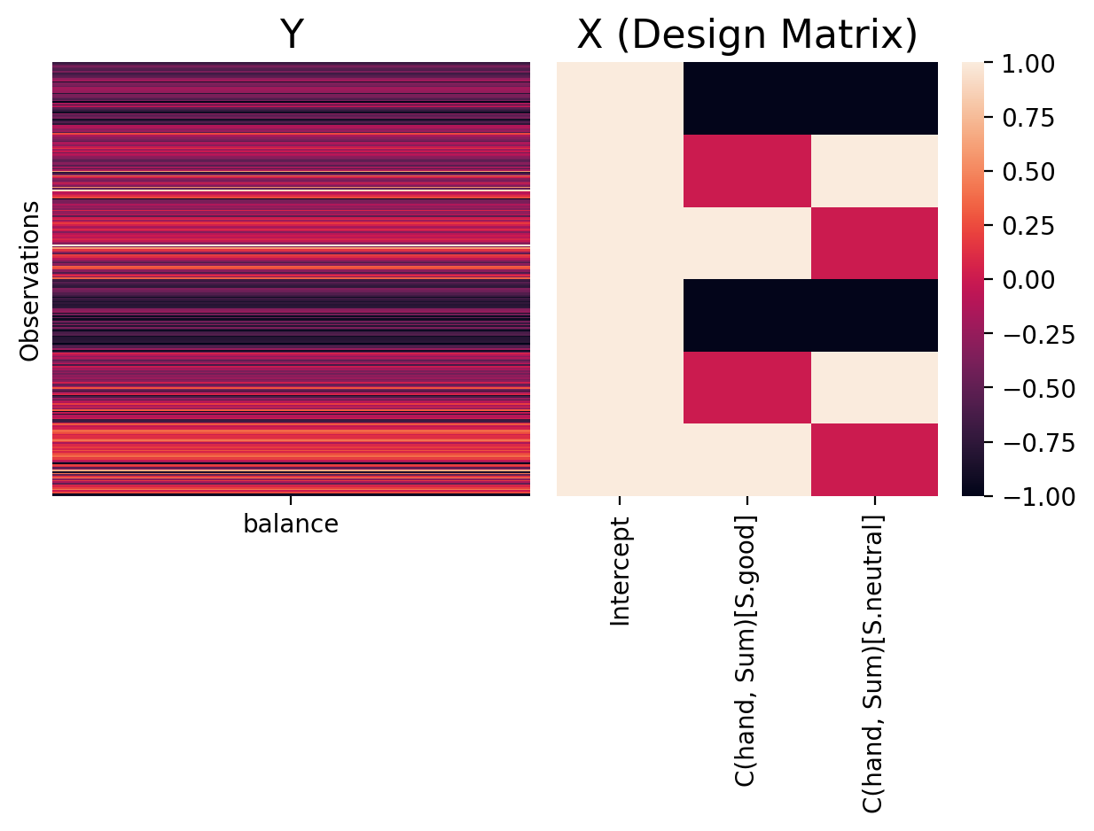
Critically for valid ANOVA tests the sum over rows of this scheme adds up to 0:
model_sum.exog.sum(axis=0)
array([300., 0., 0.])
Compare this to our treatment/dummy coding which did not!
model_a.exog.sum(axis=0)
array([300., 100., 100.])
Interpreting Parameters#
In this coding scheme parameters represent:
Intercept = the grand-mean of
balanceover all levels ofhand\(\beta_1\) = difference between the mean of
hand = 'good'and the grand-mean\(\beta_2\) = difference between the mean of
hand = 'neutral'and the grand-mean
print(results_sum.summary(slim=True))
                            OLS Regression Results
==============================================================================
Dep. Variable:                balance   R-squared:                       0.338
Model:                            OLS   Adj. R-squared:                  0.333
No. Observations:                 300   F-statistic:                     75.70
Covariance Type:            nonrobust   Prob (F-statistic):           2.70e-27
=======================================================================================================
                                          coef    std err          t      P>|t|      [0.025      0.975]
-------------------------------------------------------------------------------------------------------
Intercept                               9.7715      0.237     41.165      0.000       9.304      10.239
C(hand, Sum(omit='bad'))[S.good]        3.2549      0.336      9.696      0.000       2.594       3.916
C(hand, Sum(omit='bad'))[S.neutral]     0.5751      0.336      1.713      0.088      -0.086       1.236
=======================================================================================================

Notes:
[1] Standard Errors assume that the covariance matrix of the errors is correctly specified.
Challenge#
Using the mean for each level of hand you calculated earlier and any other values you need to calculate, use the means to recreate what each parameter estimate represents
Use print in Python or a markdown cell to write out your explanation
# Your code here
# Solution
grand_mean = np.mean([bad, good, neutral])

print(f"Intercept = Grand-mean = {grand_mean:.3f}")
print(f"B1 = Good - Grand-mean = {good - grand_mean:.3f}")
print(f"B2 = Neutral - Grand-mean = {neutral - grand_mean:.3f}")
Intercept = Grand-mean = 9.772
B1 = Good - Grand-mean = 3.255
B2 = Neutral - Grand-mean = 0.575
Orthogonal Polynomial Coding#
This form of coding uses the intercept to estimate the grand-mean (mean of means) of all levels and uses additional parameters to calculate polynomial trends across levels of the categorical variable, i.e. linear, quadratic, cubic, etc.
We can use this coding scheme with C(Student, Poly)
# Estimate model
model_poly = ols("balance ~ C(hand, Poly)", data=df.to_pandas())
results_poly = model_poly.fit()
# Print first 10 rows of the design matrix
model_poly.exog[:10, :]
array([[ 1.        , -0.70710678,  0.40824829],
       [ 1.        , -0.70710678,  0.40824829],
       [ 1.        , -0.70710678,  0.40824829],
       [ 1.        , -0.70710678,  0.40824829],
       [ 1.        , -0.70710678,  0.40824829],
       [ 1.        , -0.70710678,  0.40824829],
       [ 1.        , -0.70710678,  0.40824829],
       [ 1.        , -0.70710678,  0.40824829],
       [ 1.        , -0.70710678,  0.40824829],
       [ 1.        , -0.70710678,  0.40824829]])
# Visualize the design matrix
plot_design_matrix(model_poly, cbar=True)
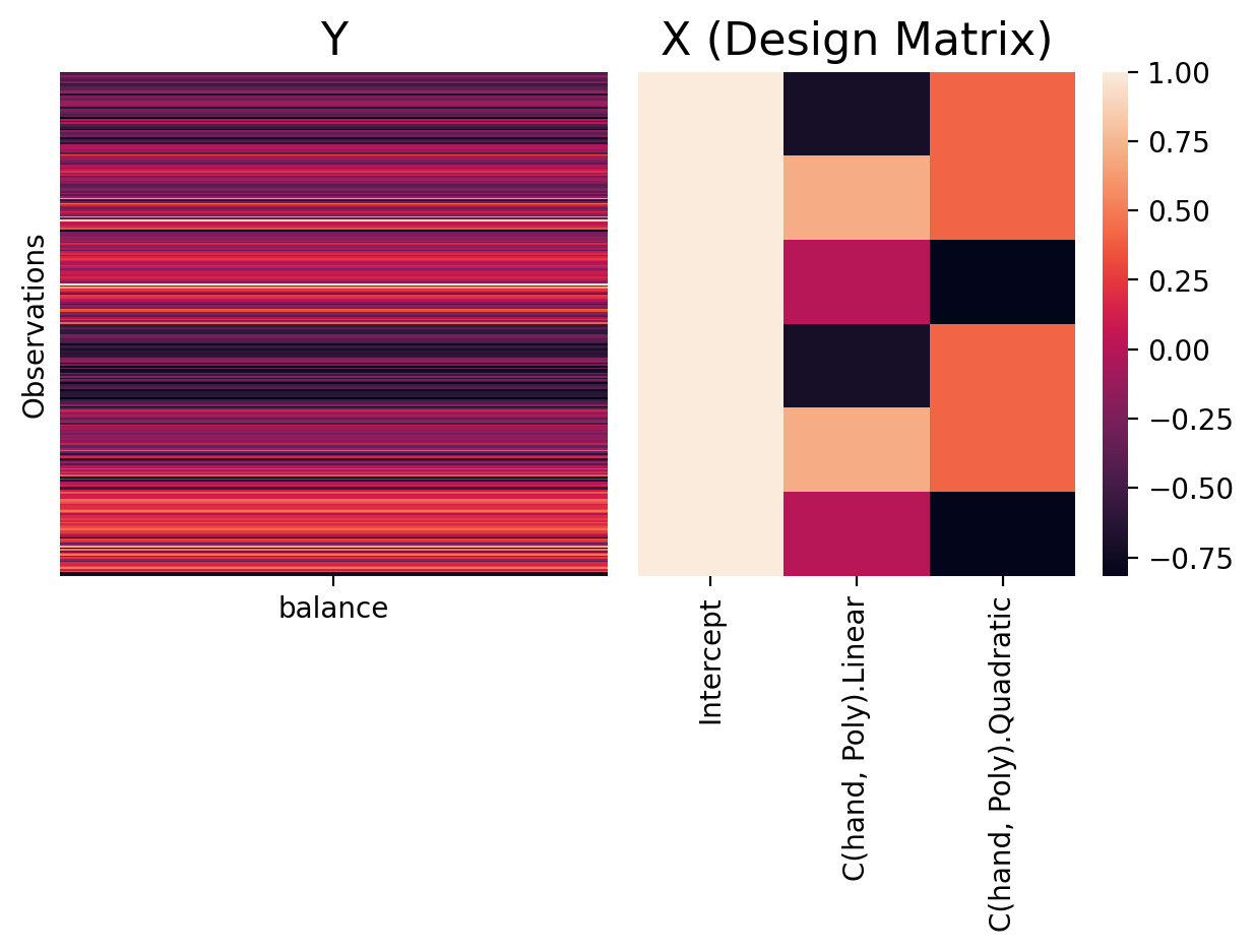
Like sum/deviation coding, polynomial contrasts are for valid ANOVA tests as the sum over rows of this scheme adds up to 0:
model_poly.exog.sum(axis=0)
array([ 3.00000000e+02, -5.06586146e-15, -1.55653268e-13])
Interpreting Parameters#
In this coding scheme parameters represent:
Intercept = the grand-mean of
balanceover all levels ofhand\(\beta_1\) = linear trend over levels of
hand\(\beta_2\) = quadratic trend over levels of
hand
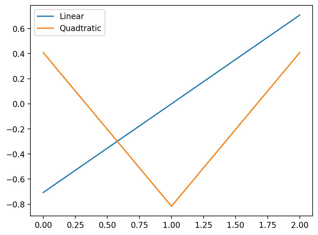
To see this more clearly let’s visualize how Poly is encoding levels of hand
# Import the Poly function which we don't normally use directly
from patsy.contrasts import Poly

# Generate a matrix using our predictor variables
poly_codes = Poly().code_without_intercept(model_poly.exog_names).matrix

poly_codes = pl.DataFrame(poly_codes,
                          schema=['linear', 'quadratic']).with_columns(
                              hand = np.array(['bad', 'good','neutral']))
The matrix above is like a “mini” design matrix mapping the levels of hand to the polynomial value
Visually if we think about each level of hand on the x-axis below we can see how the polynomial value changes:
plt.plot(poly_codes[:, 0], label='Linear')
plt.plot(poly_codes[:, 1], label='Quadtratic')
plt.legend();
print(results_poly.summary(slim=True))
                            OLS Regression Results
==============================================================================
Dep. Variable:                balance   R-squared:                       0.338
Model:                            OLS   Adj. R-squared:                  0.333
No. Observations:                 300   F-statistic:                     75.70
Covariance Type:            nonrobust   Prob (F-statistic):           2.70e-27
===========================================================================================
                              coef    std err          t      P>|t|      [0.025      0.975]
-------------------------------------------------------------------------------------------
Intercept                   9.7715      0.237     41.165      0.000       9.304      10.239
C(hand, Poly).Linear        3.1149      0.411      7.576      0.000       2.306       3.924
C(hand, Poly).Quadratic    -3.9864      0.411     -9.696      0.000      -4.796      -3.177
===========================================================================================

Notes:
[1] Standard Errors assume that the covariance matrix of the errors is correctly specified.
Challenge#
Using the mean for each level of hand you calculated earlier and the poly_codes matrix below try to recreate the value for the linear and quadratic estimates above.
Hint: Think about using np.dot…
# Use the first 2 columns of this matrix
poly_codes
| linear | quadratic | hand |
|---|---|---|
| f64 | f64 | str |
| -0.707107 | 0.408248 | "bad" |
| -1.6940e-17 | -0.816497 | "good" |
| 0.707107 | 0.408248 | "neutral" |
# Solution
linear_codes = poly_codes[:, 0].to_numpy()
linear_contrast = np.dot([bad, good, neutral], linear_codes)

quadratic_codes = poly_codes[:, 1].to_numpy()
quadratic_contrast = np.dot([bad, good, neutral], quadratic_codes)

print(f"Linear contrast: {linear_contrast:.3f}")
print(f"Quadratic contrast: {quadratic_contrast:.3f}")
Linear contrast: 3.115
Quadratic contrast: -3.986